Part 5: Scaling to 4D and Beyond

This part shows how regularizeNd extends naturally to 4-D (and higher) inputs. The concepts follow a workflow adapted to a self-contained synthetic dataset so you can run it anywhere.

Practical Goal

Build intuition for how grid size grows from 2D to 4D and beyond.
Apply per-dimension smoothness values based on signal behavior.
Use coarse-to-fine refinement to control runtime and memory.

Example Anchor

Primary script: regularizeNd/Examples/a05_example_4D_input.m

Conceptual Model

High-dimensional fitting in regularizeNd is still the same fidelity-plus-smoothness least-squares model used in lower dimensions, but grid cardinality grows multiplicatively. The key strategy is to stay coarse first, tune smoothness, then selectively refine dimensions that matter most adding points only where needed to capture variation without exploding the total grid size.

The Core Challenge of High Dimensions

Adding a dimension does not add to grid count — it multiplies it. For a grid of \(N\) points per dimension across \(d\) dimensions, the total node count is \(N^d\):

Nodes/dim	2-D	3-D	4-D	5-D
5	25	125	625	3 125
10	100	1 000	10 000	100 000
20	400	8 000	160 000	3 200 000
30	900	27 000	810 000	24 300 000

This is the curse of dimensionality for grid-based methods. The practical consequence is that you must be intentional about how many points you allocate to each dimension.

The linear system solved internally has:

columns = total grid nodes = \(\prod_i N_i\)
rows = data count + regularization equations ≫ columns (overdetermined)
nonzeros ∝ \(2^d \cdot N_\text{data}\) (for linear interpolation)

The reference 4-D example in a05_example_4D_input.m uses 30 240 grid nodes, producing a system with 250 505 rows and 2 539 252 nonzero elements, which solves in ~3.5 seconds on a 2019 laptop (32 GB RAM, i7 CPU).

The Synthetic 4-D Dataset

The synthetic response is: dens \[ w = \sin(2\pi x_1) \cdot \cos(\pi x_2) + 0.4 \, x_3^2 + 0.1 \, x_4 + \varepsilon \]

where \(\varepsilon \sim \mathcal{N}(0, 0.05^2)\), normally distributed with 0.05 standard deviation. The four inputs span different physical scales and have deliberately different levels of variation — motivating per-dimension smoothness.

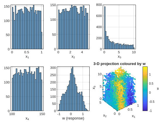
clc; clear; close all;
rng(2025);

% --- scatter data ---
N = 4000;
x1 = rand(N,1);           % [0, 1]   — fast oscillation
x2 = 5*rand(N,1);         % [0, 5]   — moderate variation
x3 = 10*rand(N,1).^2;     % [0, 10]  — nonlinear fill (denser near 0)
x4 = 100 + 50*rand(N,1);  % [100,150] — slow ramp

noise = 0.05 * randn(N,1);
w = sin(2*pi*x1) .* cos(pi*x2/5) + 0.4*(x3/10).^2 + 0.1*(x4-100)/50 + noise;

% --- inspect each input marginal ---
figure
tiledlayout(2, 3, 'TileSpacing', 'compact', 'Padding', 'compact')

inputs  = {x1, x2, x3, x4, w};
iLabels = {'x_1', 'x_2', 'x_3', 'x_4', 'w (response)'};
for k = 1:5
    nexttile
    histogram(inputs{k}, 30)
    xlabel(iLabels{k}); grid on
end

nexttile
scatter3(x1, x2, x3, 12, w, 'filled')
xlabel('x_1'); ylabel('x_2'); zlabel('x_3')
h = colorbar; ylabel(h, 'w')
title('3-D projection coloured by w')

The x3 marginal is right-skewed because we drew from a squared-uniform distribution. This will motivate non-uniform grid spacing in that dimension later.

Coarse Grid: Getting Oriented

Always start coarse. A coarse grid tells you whether the smoothness values are in the right ballpark before committing to a fine grid.

% --- coarse grid (fast) ---
x1GridCoarse = linspace(0,   1,   8);
x2GridCoarse = linspace(0,   5,   9);
x3GridCoarse = linspace(0,  10,   10);   % uniform for now
x4GridCoarse = linspace(100,150,  6);
xGridCoarse = {x1GridCoarse, x2GridCoarse, x3GridCoarse, x4GridCoarse};

% per-dimension smoothness:
%   x1 has fast oscillation → small smoothness
%   x2 moderate              → moderate
%   x3 slow quadratic        → larger smoothness is fine
%   x4 very slow ramp        → largest smoothness
smoothness = [1e-3, 1e-3, 1e-2, 2e-2];

tic
wGridCoarse = regularizeNd([x1,x2,x3,x4], w, xGridCoarse, smoothness);
fprintf('Coarse grid  (%d nodes)  solve time: %.2f s\n', numel(wGridCoarse), toc)

wFuncCoarse = griddedInterpolant(xGridCoarse, wGridCoarse);

Coarse grid  (4320 nodes)  solve time: 0.14 s

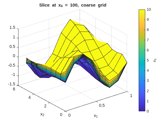
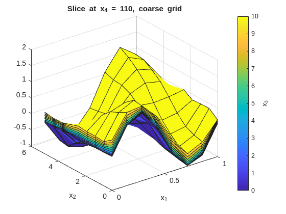
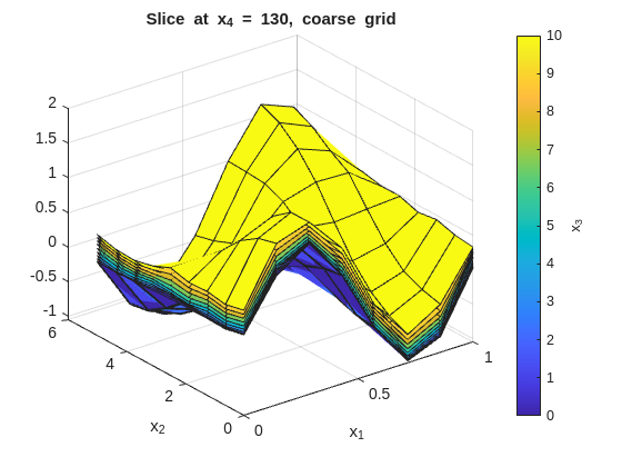
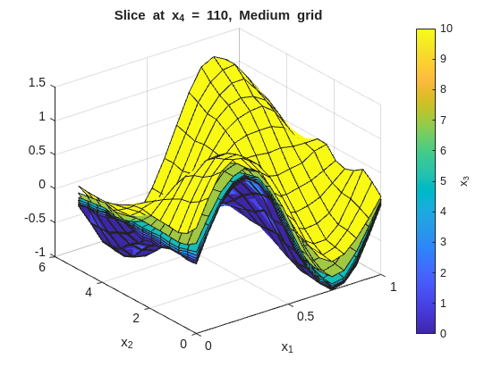
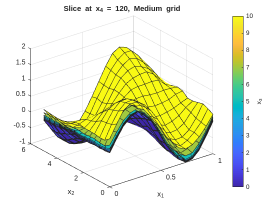
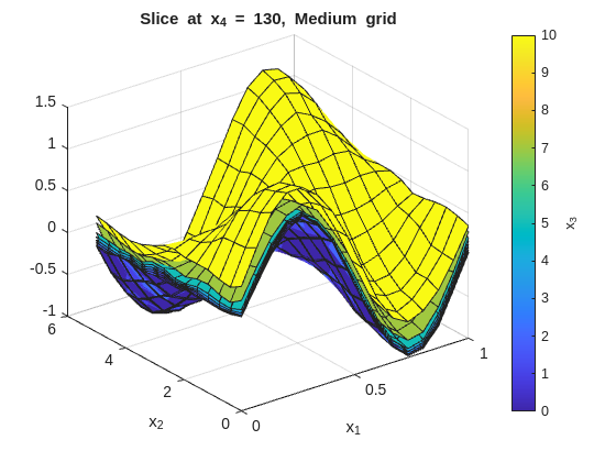
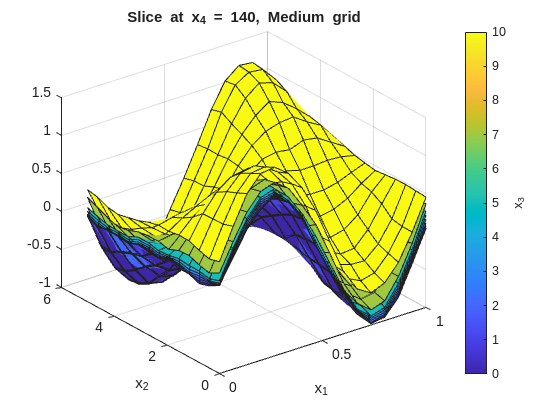
Inspect the fit with x_1 on the x-axis and x_2 on the y-axis. Each figure fixes one x_4 value and overlays surfaces across the x_3 slices:

% --- 2-D slice: vary x1 and x2, fix x3 and x4 ---
onesMatrix = ones(numel(x1GridCoarse), numel(x2GridCoarse))';
for i = 1:numel(x4GridCoarse)
  for j = 1:numel(x3GridCoarse)
    wSlice = squeeze(wGridCoarse(:,:,j,i))';
    if j == 1
      titleStr = sprintf("Slice at x_4 = %g, coarse grid", x4GridCoarse(i));
      figure("Name", titleStr);
      surf(x1GridCoarse, x2GridCoarse, wSlice, x3GridCoarse(j)*onesMatrix);
      hold on;
      ylabel(colorbar,"x_3");
      xlabel('x_1'); 
      ylabel('x_2');
      title(titleStr);
    else
      surf(x1GridCoarse, x2GridCoarse, wSlice, x3GridCoarse(j)*onesMatrix);
    end
  end
end

Refine One Dimension at a Time

Increase resolution only in the dimension where the slice shows unresolved detail. You can see this from high residuals or local large gradients even with large smoothness.

% --- moderate grid: refine x1 and x2 where variation is fastest ---
x1GridMedium = linspace(0,   1,  16);
x2GridMedium = linspace(0,   5,  14);
x3GridMedium = [0, 1, 2, 3, 4, 5, 7, 10];   % denser near 0 to match data fill
x4GridMedium = linspace(100,150,  6);
gridMedium = {x1GridMedium, x2GridMedium, x3GridMedium, x4GridMedium};

fprintf('Medium grid node count: %d\n', prod(cellfun(@numel,gridMedium)))

tic
wGridMedium = regularizeNd([x1,x2,x3,x4], w, gridMedium, smoothness);
fprintf('Medium grid  (%d nodes)  solve time: %.2f s\n', numel(wGridMedium), toc)

wFuncMedium = griddedInterpolant(gridMedium, wGridMedium);

Medium grid node count: 10752
Medium grid  (10752 nodes)  solve time: 0.39 s

Notice the non-uniform x3GridMedium spacing. Because x3 data is denser near 0, placing more grid nodes there improves fidelity in the data-rich region while keeping node count low elsewhere.

% --- 2-D slice: vary x1 and x2, fix x3 and x4 ---
onesMatrix = ones(numel(x1GridMedium), numel(x2GridMedium))';
for i = 1:numel(x4GridMedium)
  for j = 1:numel(x3GridMedium)
    wSlice = squeeze(wGridMedium(:,:,j,i))';
    if j == 1
      titleStr = sprintf("Slice at x_4 = %g, Medium grid", x4GridMedium(i));
      figure("Name", titleStr);
      surf(x1GridMedium, x2GridMedium, wSlice, x3GridMedium(j)*onesMatrix);
      hold on;
      ylabel(colorbar,"x_3");
      xlabel('x_1'); 
      ylabel('x_2');
      title(titleStr);
    else
      surf(x1GridMedium, x2GridMedium, wSlice, x3GridMedium(j)*onesMatrix);
    end
  end
end

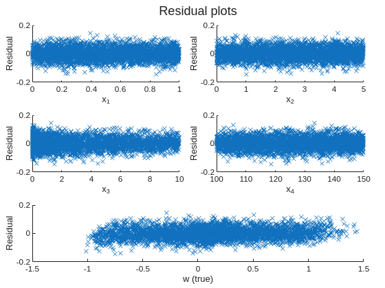
Checking Residuals

Residuals are the quickest global quality indicator. Look for patterns in the residuals versus each input dimension or versus the true response — systematic structure indicates underfitting (grid too coarse or smoothness too large), while residuals that are roughly zero with no heavy tails indicate the smoothness and grid combination is adequate.

In this data set, the residuals from the medium grid fit should be roughly zero with no obvious patterns, indicating that the grid resolution and smoothness are capturing the main structure of the function without overfitting the noise. TIP: In other data sets, with bias present or high noise, some patterns or large residuals is to be expected. A decent fit rather than a great fit is the compromise when dealing with noisy or biased data.

resid = w - wFuncMedium(x1, x2, x3, x4);

figure("Name", "Residuals")
tl = tiledlayout('TileSpacing', 'compact', 'Padding', 'compact');
title(tl, "Residual plots")

nexttile
scatter(x1, resid,"x");
xlabel('x_1'); ylabel('Residual')
nexttile
scatter(x2, resid,"x");
xlabel('x_2'); ylabel('Residual')
nexttile
scatter(x3, resid,"x");
xlabel('x_3'); ylabel('Residual')
nexttile
scatter(x4, resid,"x");
xlabel('x_4'); ylabel('Residual')
nexttile([1,2])
scatter(w, resid,"x");
xlabel('w (true)'); ylabel('Residual')

Comparing Slices Across Smoothness Values

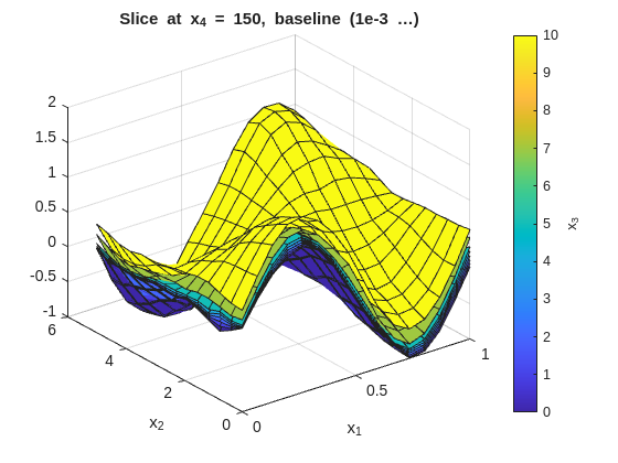
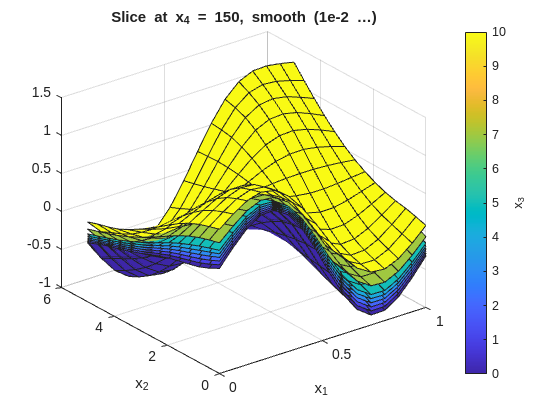
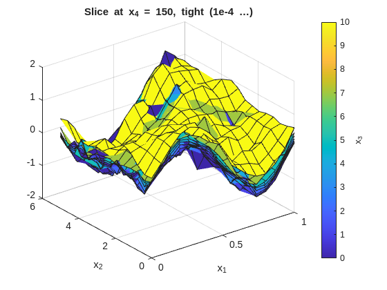
The same slice-plot approach can be reused to compare several smoothness settings. Here the page regenerates the x_1-x_2 slice families for three representative smoothness choices:

smoothnessValues = {
    [1e-3, 1e-3, 1e-2, 2e-2],   % baseline
    [1e-2, 1e-2, 1e-1, 2e-1],   % 10× smoother
    [1e-4, 1e-4, 1e-3, 2e-3],   % 10× tighter
};
labels = {'baseline (1e-3 …)', 'smooth (1e-2 …)', 'tight (1e-4 …)'};

for k = 1:3
  wG = regularizeNd([x1,x2,x3,x4], w, gridMedium, smoothnessValues{k});

  onesMatrix = ones(numel(x1GridMedium), numel(x2GridMedium))';
  x4SliceIndex = numel(x4GridMedium);
  for j = 1:numel(x3GridMedium)
    wSlice = squeeze(wG(:,:,j,x4SliceIndex))';
    if j == 1
      titleStr = sprintf("Slice at x_4 = %g, %s", x4GridMedium(x4SliceIndex), labels{k});
      figure("Name", titleStr);
      surf(x1GridMedium, x2GridMedium, wSlice, x3GridMedium(j)*onesMatrix);
      hold on;
      ylabel(colorbar,"x_3");
      xlabel('x_1');
      ylabel('x_2');
      title(titleStr);
    else
      surf(x1GridMedium, x2GridMedium, wSlice, x3GridMedium(j)*onesMatrix);
    end
  end
end

The tight (low smoothness) plots will show more local variation across the x_3 overlays. The smooth (high smoothness) plots will flatten those differences. The baseline should preserve the main structure without overreacting to noise.

Grid Design Rules of Thumb

These rules follow directly from the a05_example_4D_input.m comments and workflow:

Start coarse (5–10 nodes/dim) and verify the smoothness range before refining.
Non-uniform spacing where the data or function has concentrated structure — denser nodes in the dense-data region, sparser in sparse regions.
Per-dimension smoothness — assign smaller values to fast-varying dimensions and larger values to slow-varying ones.
Budget the node product — for a direct solver, a practical ceiling is roughly 1e6–10e6 total grid nodes before switching to an iterative solver (see Part 7). This number will depend on your computer resources (RAM and CPU). 1e6–10e6 is a rough orientation for a modern laptop with 32 GB of RAM and 1 min solve time; adjust downward if you have less memory or slower CPU.
Residuals before slices — a bad residual histogram reveals a grid/smoothness problem faster than any visual surface inspection.
Grid must span the data — regularizeNd throws an error if any data point falls outside xGrid. Add a small buffer if using min or max ever fails: linspace(min(x)-eps(min(x)), max(x)+eps(max(x)), N).
Different number of nodes per dimension — When working with higher-dimensional inputs, having
different number of nodes per dimension will reveal errors in indexing or array reshaping that might otherwise be hidden if all dimensions have the same node count. Using the same number of nodes in each dimension can mask bugs in how the multi-dimensional arrays are being indexed or reshaped; varying the node counts per dimension helps catch these issues early.

Checklist Before Part 6

You have computed the total grid node count and it is within your solver budget. i.e. It solves in a reasonable time without exhausting memory.
You have assigned per-dimension smoothness values proportional to observed variation rate.
You have confirmed residuals are symmetric and near pattern free..
You have compared at least two smoothness levels to confirm the baseline choice is stable.

Part 6: Constraints and Mappings