Part 6: Constraints and Mappings

This part covers two powerful capabilities that go beyond the basic regularizeNd call: applying inequality constraints to the lookup table output, and remapping input variables to a new coordinate space before fitting.

Practical Goal

Apply monotonic and bounded-output constraints to regularized lookup tables.
Understand matrix-form constrained solving with regularizeNd building blocks.
Use input-variable mappings to improve fit behavior on uneven domains.

Example Anchor

Primary script: regularizeNd/Examples/a06_constraint_and_mapping_example.m

Download the example data file a06_constraints_and_mapping.mat to run this script.

Why Constraints Matter

The unconstrained solver minimizes a weighted sum of fidelity and smoothness and is completely agnostic about the shape of the resulting lookup table. Two common engineering requirements break that assumption:

Monotonicity — the output should be non-decreasing along a given dimension (think efficiency maps, calibration curves, throttle response).
Bounded output — the table values must stay above (or below) a physical limit.

Both are linear inequality constraints of the form \(A \mathbf{y}_\text{grid} \leq \mathbf{b}\).

The Matrix Formulation

regularizeNd solves a least-squares problem inside, but you can access the individual matrices with regularizeNdMatrices:

[Afidelity, Lreg] = regularizeNdMatrices(x, xGrid, smoothness, interpMethod)

Afidelity maps grid values to predicted outputs at each data point. Lreg is a cell array of second-derivative penalty matrices, one per dimension. Stack them and you have the full system:

\[ \min_{\mathbf{y}_\text{grid}} \frac{1}{2} \left\| C \mathbf{y}_\text{grid} - \mathbf{d} \right\|_2^2 \quad \text{subject to} \quad A \mathbf{y}_\text{grid} \leq \mathbf{b} \]

where

\[ C = \begin{bmatrix} A_\text{fidelity} \\ L_\text{reg} \end{bmatrix}, \qquad \mathbf{d} = \begin{bmatrix} \mathbf{y}_\text{data} \\ \mathbf{0} \end{bmatrix}. \]

Two solvers can handle this system:

Solver	Requires	Notes
`lsqConstrainedAlternative`	base MATLAB	Bundled with regularizeNd; convergence less robust
`lsqlin`	Optimization Toolbox	More robust; supports equality constraints

Monotonic Constraint

monotonicConstraint builds the \(A\), \(\mathbf{b}\) pair for a monotonically-increasing constraint across a chosen dimension:

[Amonotonic, bMonotonic] = monotonicConstraint(xGrid)            % dimension 1 (default)
[Amonotonic, bMonotonic] = monotonicConstraint(xGrid, dim)       % specific dimension
[Amonotonic, bMonotonic] = monotonicConstraint(xGrid, dim, dxMin) % enforce minimum step

For a monotonically decreasing constraint negate the matrix: use (-Amonotonic, bMonotonic).

a06_constraint_and_mapping_example Workflow

Load and Clean the Data

For what we are going to do, we need to discard \(y\le 0\).

clc; clear; close all;
load('a06_constraints_and_mapping.mat','x','y');
index = y<=0;
x(index)=[];
y(index)=[];

Examine the Data

x to y is highly nonlinear. Specifically note the sudden and large changes in y at x=6 and x=6.45.

screenSize = get(groot,'ScreenSize');
figurePosition = screenSize(3:4)*0.1;
% figureSize = screenSize(3:4)*0.8;
figureSize = [800 600];
figurePositionAndSize = [figurePosition figureSize];
figure('Position',figurePositionAndSize)
scatter(x,y)
xlabel('x')
ylabel('y')
set(gca,'yscale','log')
grid on;
title('Examining Data')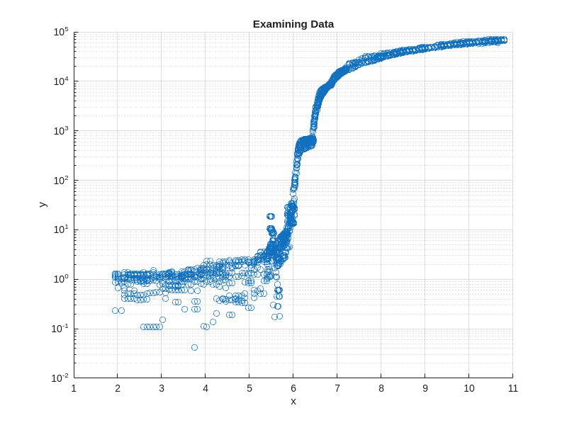

Map x to a New Space for a Smoother Map

The mapping is created manually and best explained via the video below.

The idea is to make all sections of the data the same slope, \(\frac{\Delta y}{\Delta x}\), or at least a similar slope. See the video on how I get a rough idea of the sections of the data. pchip interpolation is used because it is the smoothest interpolant that guarantees monotonic interpolation (aka no oscillations) in the mapping; a 1 to 1 mapping (1 x point maps to only 1 xNew point) is desired/required. The akima interpolation method does not always give a monotonic interpolation.

load('a06_constraints_and_mapping.mat','xValues','yValues')
desiredSlope = 1; % arbitrarily chosen
xDifference = diff(xValues);

% calculate the semilog slope
semilogSlope = diff(log10(yValues))./xDifference;

% scale slope in each section to the desired slope
xMapping = nan(size(xValues));
xMapping(1) = min(x);
for iX = 2:length(xMapping)
    xMapping(iX) = xMapping(iX-1) + semilogSlope(iX-1)./desiredSlope.*xDifference(iX-1);
end

mapping = griddedInterpolant(xValues, xMapping,'pchip','linear');

figure('Position',figurePositionAndSize)
fplot(@(x) mapping(x),[min(x), max(x)])
xlabel('x')
ylabel('xMapped')
title('Monotonic, 1 to 1 Mapping of x to xMapped')


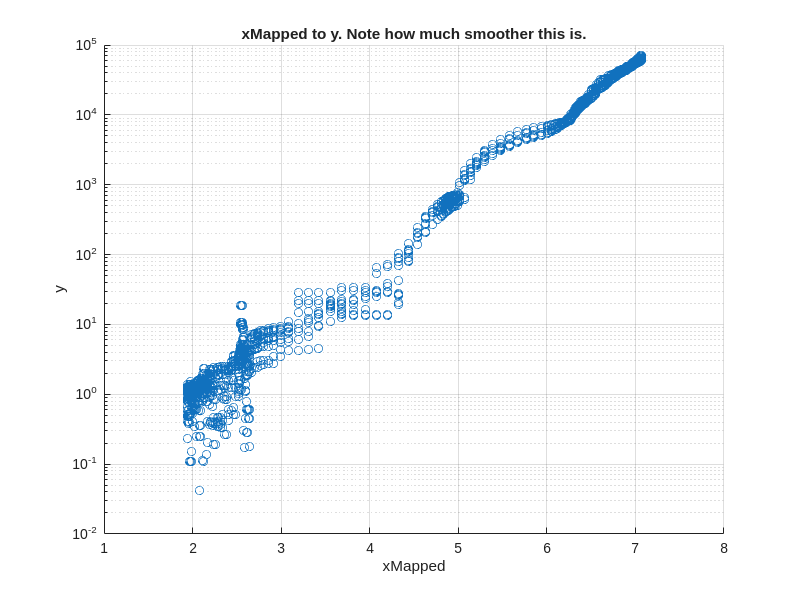
% plot new input to output
xMapped = mapping(x);
figure('Position',figurePositionAndSize)
scatter(xMapped, y)
xlabel('xMapped')
ylabel('y')
set(gca,'yscale','log')
grid on;
title('xMapped to y. Note how much smoother this is.')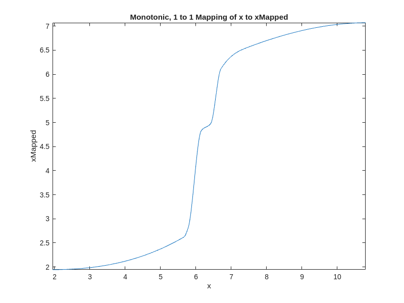

Setup Fidelity and Regularization Matrices

Set up an xGrid and then map it to the new xMapped space. The fitting will be done in the mapped space.
y is converted to log10 space because log10(y) is smoother than y.
Call regularizeNdMatrices. Get the fidelity matrix, Cfidelity, and the regularization matrix, Lregularization (in other cases, Lregularization is “matrices” if there is more than one input).
Combine the fidelity matrix, Cfidelity, and the regularization matrix, Lregularization, into one composite matrix, C.
Create the corresponding vector to C, d.

xGrid = {linspace(min(x),max(x),1000)};
xGridMapped = {mapping(xGrid{:})};
yLog10 = log10(y);
smoothness = 5e-4;

[Cfidelity, Lregularization] = regularizeNdMatrices(xMapped, xGridMapped, smoothness);
C = vertcat(Cfidelity,Lregularization{:}); % note this line of code works even if Lregularization has more than one cell

dFidelity = yLog10;
dRegularization = zeros(size(C,1)-size(Cfidelity,1),1);
d = vertcat(dFidelity, dRegularization);

Setup the Constraint Matrix

In this case, the desired constraint is that the lookup table is monotonically increasing. Also, the bound is that no value in the final table is less than 1e-2 in original y units. Since we solve for yLog10Grid, the lower bound is imposed in log space as yLog10Grid >= log10(1e-2).

The constraints are formed as inequalities like this:

\[ A*y_{\log 10,Grid} \le b \]

    % Monotonic constraint matrix
    [Amonotonic,bMonotonic] = monotonicConstraint(xGrid);
    
    nGridPoints = length(xGrid{1});
    yMin = 1e-2;
    
    % Bound constraint matrix
    Abound = sparse(nGridPoints,nGridPoints);
    Abound = spdiags(-ones(nGridPoints,1),0,Abound);
    
    % bound constraint vector
    bBound = -log10(yMin) * ones(size(Abound,1),1);
    
    % Composite constraint matrix and vector
    A = vertcat(Amonotonic, Abound);
    b = vertcat(bMonotonic, bBound);

Solve for the lookup table Using lsqConstrainedAlternative

Using the provided solver lsqConstrainedAlternative to find the lookup table yGrid1.

Create a function for use in evaluation.

    tic;
    yLog10Grid1 = lsqConstrainedAlternative(C,d,A,b);
    toc;
    yLog10GridFunction1 = griddedInterpolant(xGridMapped, yLog10Grid1,'linear');
    yFunction1 = @(x) 10.^yLog10GridFunction1(mapping(x));

Elapsed time is 0.450783 seconds.

Solve for lookup table Using lsqlin

Using the lsqlin solver has advantages. It has more flexibility but the Optimization Toolbox is required. lsqlin can handle inequality, equality, and bound constraints. In some cases lsqlin won’t converge when lsqConstrainedAlternative does. lsqlin can handle large sparse problems while lsqConstrainedAlternative is limited to smaller problems.

    % make sure lsqlin exists. If it doesn't warn the user they don't have the optimization toolbox
    if license('test', 'optimization_toolbox')
        tic;
        options = optimoptions('lsqlin', 'Display', 'iter-detailed');
        yLog10Grid2 = lsqlin(C,d,A,b,[],[],[],[],[],options);
        toc;
        yLog10GridFunction2 = griddedInterpolant(xGridMapped, yLog10Grid2,'linear');
        yFunction2 = @(x) 10.^yLog10GridFunction2(mapping(x));
    else
        warning('Optimization Toolbox is not installed. Use lsqConstrainedAlternative or another provided linear solver.')

        yFunction2 = @(x) nan(size(x));
    end

Warning: Optimization Toolbox is not installed. Use lsqConstrainedAlternative or another provided linear solver.

Plot the Results

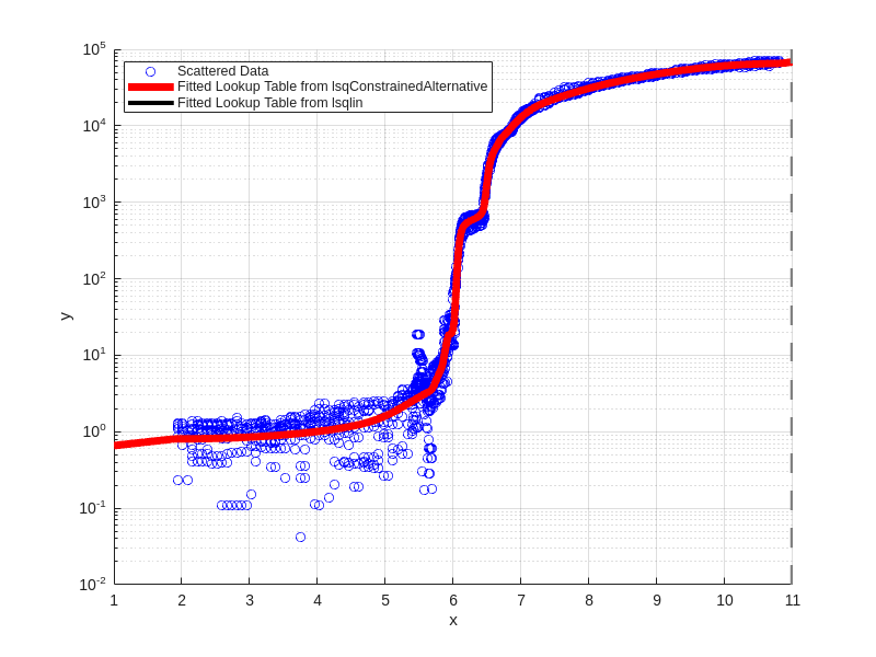
The fitted lookup tables work great in both the lsqConstrainedAlternative and lsqlin cases.

Note that both fits are monotonically increasing and greater than or equal to 1e-2.

figure('Position',figurePositionAndSize)
scatter(x,y,'b');
hold on;
fplot(yFunction1,xlim,'r','linewidth',5);
fplot(yFunction2,xlim,'k','linewidth',3);
xlabel('x')
ylabel('y')
set(gca,'yscale','log')
grid on;
legend({'Scattered Data','Fitted Lookup Table from lsqConstrainedAlternative', 'Fitted Lookup Table from lsqlin'},'location','best')

Checklist Before Leaving This Part

Can you assemble C and d manually from regularizeNdMatrices output?
Does lsqConstrainedAlternative solve and return a non-decreasing table?
Have you verified the difference vector diff(yGrid) is everywhere ≥ 0?
If the raw data has a steep section, have you tried a log-axis or a piecewise mapping?

Part 7: Iterative Solvers and Memory Strategy