Part 4: Boundary Behavior and Convex Hull

Back to regularizeNd series home

Previous: Part 3

This part explains why regularized lookup tables remain well-behaved near sparse boundaries while standard scattered interpolation can collapse.

Practical Goal

1. Understand why convex-hull geometry can break scattered interpolation.
2. Compare boundary behavior between scatteredInterpolant and regularizeNd.
3. Build intuition for why regularization stabilizes sparse edge regions.

Example Anchor

Primary script: regularizeNd/Examples/a04_example_scattered_data_near_convex_hull.m

Conceptual Model

scatteredInterpolant depends on Delaunay triangles and can become unstable when triangles near the convex hull are long and sliver-like. regularizeNd instead solves a global least-squares system with a smoothness penalty, so sparsely supported regions are governed by nearby trend continuation rather than local triangulation artifacts.

The Dataset: A Deliberately Pathological Point Cloud

The example data is a synthetic 2-D point cloud shaped like a lens:

• Two arcs (upper and lower) tracing portions of a unit circle.
• A thin horizontal bar connecting them through the middle.

This geometry is designed so that the Delaunay triangulation used internally by scatteredInterpolant produces extremely sliver-like triangles in the nearly-empty corners of the convex hull. The true underlying surface is the paraboloid \(z = x^2 + y^2\).

clc; clear; close all;


% --- build the lens-shaped point cloud ---
t  = 0.4*pi : 0.02 : 0.6*pi;
x1 = cos(t)';    y1 = sin(t)' - 1.02;   % bottom arc
x2 = x1;         y2 = -y1;              % top arc (mirror)
x3 = linspace(-0.3, 0.3, 16)';  y3 = zeros(16,1);  % horizontal bar

x = [x1; x2; x3];
y = [y1; y2; y3];
z = x.^2 + y.^2;   % true paraboloid

k = convhull(x, y);

figure('Color', 'w', 'Position', [100, 100, 760, 520])
scatter(x, y, 54, z, 'filled', ...
   'MarkerEdgeColor', [0.15, 0.15, 0.15], 'LineWidth', 0.3, 'MarkerFaceAlpha', 0.95)
hold on
plot(x(k), y(k), '-', 'Color', [0.10, 0.10, 0.10], 'LineWidth', 1.8)
colormap(turbo)
cb = colorbar;
cb.Label.String = 'z = x^2 + y^2';
xlabel('x'); ylabel('y')
title('Point cloud with convex hull')
set(gca, 'FontSize', 11, 'LineWidth', 0.8)
grid on; box on
axis equal tight
xlim([-0.35, 0.35]); ylim([-0.12, 0.12])

Notice that the convex hull covers a much larger area than the data itself. The four corner regions are almost entirely unsupported.

Why scatteredInterpolant Fails Near This Hull

scatteredInterpolant builds a Delaunay triangulation of the input points and then interpolates within each triangle. In the corner regions the triangles are sliver-shaped — connecting points that are far apart and nearly collinear. Interpolation inside a sliver triangle amplifies numerical error, leading to wildly wrong surface values near the hull boundary.

regularizeNd Does Not Fail Here

regularizeNd is not an interpolant. It solves a weighted least-squares problem:

\[ \min_{\mathbf{y}_\text{grid}} \left\| A_\text{fidelity}\,\mathbf{y}_\text{grid} - \mathbf{z}_\text{data} \right\|^2 + \lambda^2 \left\| L\,\mathbf{y}_\text{grid} \right\|^2 \]

Where:

• \(\mathbf{y}_\text{grid}\) is the unknown vector of grid values to solve for.
• \(A_\text{fidelity}\) maps grid values to the sample locations (data-fit operator).
• \(\mathbf{z}_\text{data}\) is the vector of measured data values at the sample points.
• \(L\) is the regularization operator (for example, finite-difference derivatives on the grid).
• \(\lambda\) is the smoothness weight that balances data fit and regularization.

Where data is sparse the regularization term takes over and enforces a smooth continuation of whatever trend exists nearby. It does not need a well-shaped triangulation.

Side-by-Side Comparison

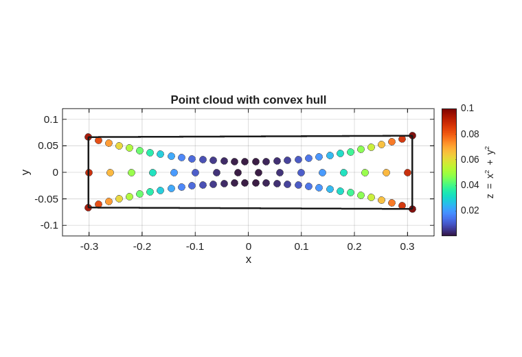
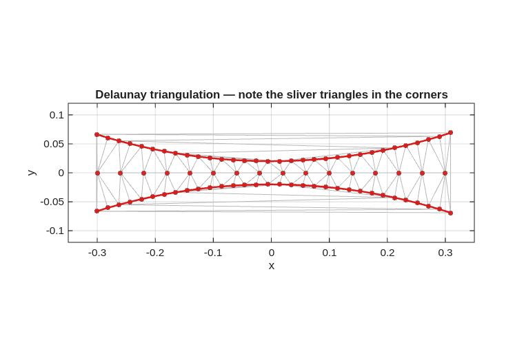
% --- build point cloud (same as above, in same script session) ---
t  = 0.4*pi : 0.02 : 0.6*pi;
x1 = cos(t)';    y1 = sin(t)' - 1.02;
x2 = x1;         y2 = -y1;
x3 = linspace(-0.3, 0.3, 16)';  y3 = zeros(16,1);
x = [x1; x2; x3];
y = [y1; y2; y3];
z = x.^2 + y.^2;

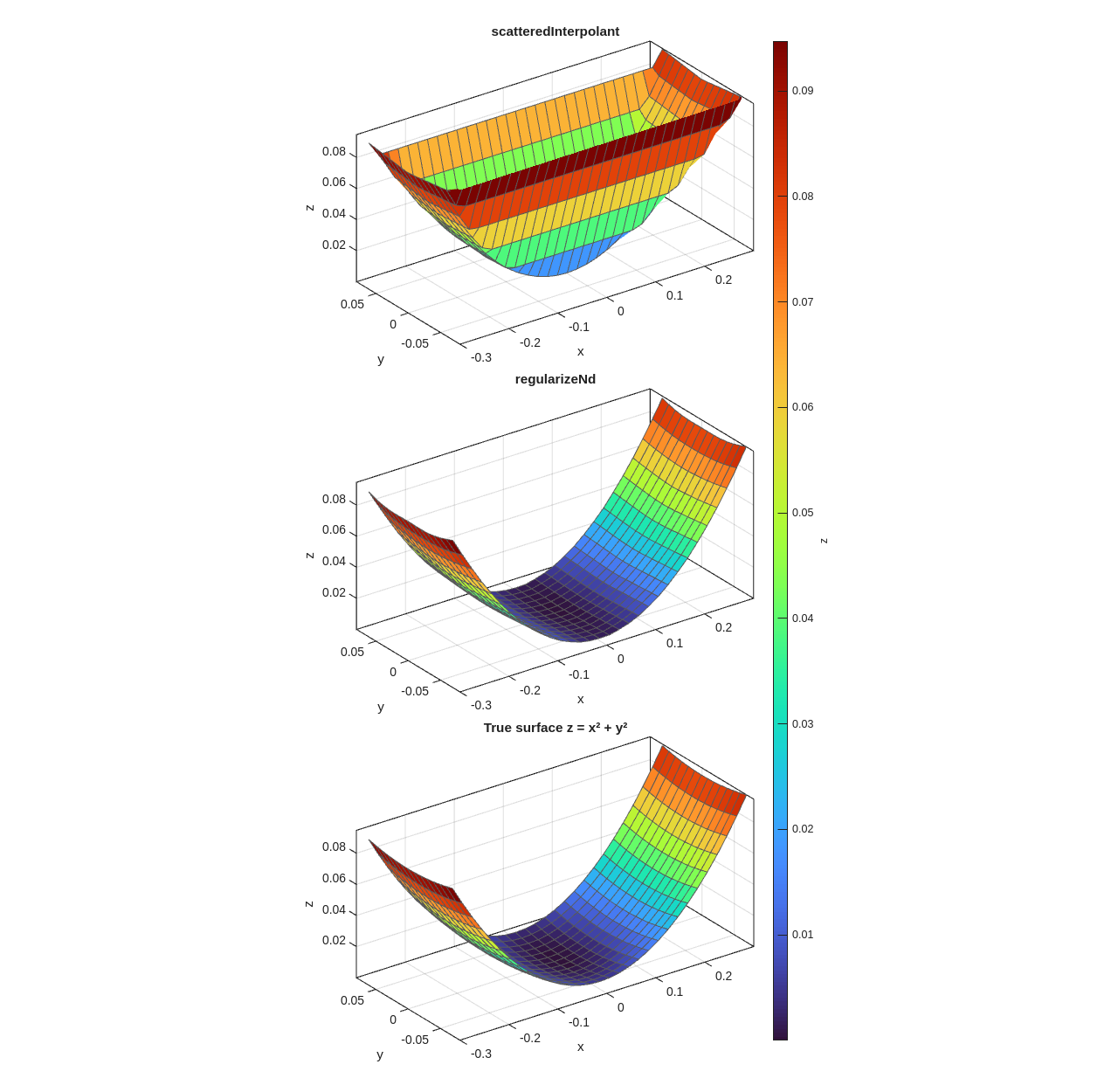
% --- scatteredInterpolant ---
F = scatteredInterpolant(x, y, z);

% --- regularizeNd ---
xGrid = {linspace(min(x)-eps(min(x)), max(x)+eps(max(x)), 20), ...
         linspace(min(y)-eps(min(y)), max(y)+eps(max(y)), 21)};
zGrid = regularizeNd([x,y], z, xGrid, [0.001, 0.005], 'linear');
F2 = griddedInterpolant(xGrid, zGrid, 'linear');

% --- evaluation grid ---
[xi, yi] = ndgrid(-0.3:0.02:0.3, -0.0688:0.01:0.0688);
zi_scattered  = F(xi, yi);
zi_regularize = F2(xi, yi);
zi_true       = xi.^2 + yi.^2;

zmin = min(zi_true(:));
zmax = max(zi_true(:));

figure('Color', 'w', 'Position', [100, 100, 1280, 1250])
tl = tiledlayout(3, 1, 'TileSpacing', 'compact', 'Padding', 'compact');
colormap(turbo(256))

nexttile
s1 = surf(xi, yi, zi_scattered, 'EdgeColor', [0.35, 0.35, 0.35], 'LineWidth', 0.2);
title('scatteredInterpolant')
xlabel('x'); ylabel('y'); zlabel('z')
caxis([zmin, zmax])
xlim([-0.3, 0.3]); ylim([-0.08, 0.08]); zlim([zmin, zmax])
view(-36, 26)
daspect([1, 0.55, 0.35])
set(gca, 'FontSize', 10, 'LineWidth', 0.8)
grid on; box on

nexttile
s2 = surf(xi, yi, zi_regularize, 'EdgeColor', [0.35, 0.35, 0.35], 'LineWidth', 0.2);
title('regularizeNd')
xlabel('x'); ylabel('y'); zlabel('z')
caxis([zmin, zmax])
xlim([-0.3, 0.3]); ylim([-0.08, 0.08]); zlim([zmin, zmax])
view(-36, 26)
daspect([1, 0.55, 0.35])
set(gca, 'FontSize', 10, 'LineWidth', 0.8)
grid on; box on

nexttile
s3 = surf(xi, yi, zi_true, 'EdgeColor', [0.35, 0.35, 0.35], 'LineWidth', 0.2);
title('True surface z = x² + y²')
xlabel('x'); ylabel('y'); zlabel('z')
caxis([zmin, zmax])
xlim([-0.3, 0.3]); ylim([-0.08, 0.08]); zlim([zmin, zmax])
view(-36, 26)
daspect([1, 0.55, 0.35])
set(gca, 'FontSize', 10, 'LineWidth', 0.8)
grid on; box on

cb = colorbar;
cb.Layout.Tile = 'east';
cb.Label.String = 'z';

The scatteredInterpolant surface spikes dramatically near the convex hull corners. The regularized surface follows the paraboloid trend smoothly even in the corner regions where no data exists.

Inspecting the Triangulation

The reason for the failure is visible in the Delaunay triangulation:

t  = 0.4*pi : 0.02 : 0.6*pi;
x1 = cos(t)';    y1 = sin(t)' - 1.02;
x2 = x1;         y2 = -y1;
x3 = linspace(-0.3,0.3,16)';  y3 = zeros(16,1);
x = [x1; x2; x3];
y = [y1; y2; y3];

dt = delaunayTriangulation(x, y);

figure('Color', 'w', 'Position', [100, 100, 760, 520])
triplot(dt, 'Color', [0.72 0.72 0.72], 'LineWidth', 0.7)
hold on
scatter(x, y, 22, [0.84, 0.15, 0.15], 'filled', ...
   'MarkerEdgeColor', [0.30, 0.08, 0.08], 'LineWidth', 0.25)
plot(x1, y1, '-', 'Color', [0.85, 0.10, 0.10], 'LineWidth', 1.8)
plot(x2, y2, '-', 'Color', [0.85, 0.10, 0.10], 'LineWidth', 1.8)
axis equal tight
xlim([-0.35, 0.35]); ylim([-0.12, 0.12])
set(gca, 'FontSize', 11, 'LineWidth', 0.8)
grid on; box on
title('Delaunay triangulation — note the sliver triangles in the corners')
xlabel('x'); ylabel('y')

Triangles inside the red arc boundaries are reasonably shaped. Outside them, the triangles connect remote points across nearly-empty regions — linear interpolation inside a sliver produces values that have little to do with the underlying surface.

Key Takeaways

	scatteredInterpolant	regularizeNd
Uses triangulation	Yes	No
Requires well-sampled hull interior	Yes	No
Behavior near sparse hull boundary	Can spike/degrade	Smooth regularized continuation
Is it an interpolant?	Yes — passes through every point	No — weighted least-squares fit
Control over boundary behavior	None	Via smoothness parameter

What Controls Edge Behavior in regularizeNd

1. Smoothness magnitude — the dominant control. Away from the the data, the solution is essentially a smooth continuation of nearby trends.
2. Derivative order — second-order regularization enforces near-linear continuation; a first-order variant would enforce near-constant continuation.
3. Grid extent relative to data coverage — keeping the grid tightly bounded by the data limits how far the model is asked to extrapolate.
4. Anisotropic smoothness — per-dimension smoothness values (as used above: [0.001, 0.005]) let you tune propagation differently along each axis.

Boundary Tuning Protocol

1. Fix interpolation mode ('linear' is the recommended baseline).
2. Start with equal per-dimension smoothness and compare with the true or reference surface.
3. If boundary behavior is implausible, increase smoothness in the offending dimension.
4. Re-check interior residuals after any smoothness increase — over-smoothing will degrade the interior fit.

Checklist Before Part 5

• You have plotted the data geometry and identified the convex hull.
• You have compared your method against a known reference surface where one exists.
• You have inspected the boundary and corner regions explicitly, not just the dense interior.
• You have selected a smoothness value that gives plausible behavior across the full grid domain.

Next

Part 5: Scaling to 4D and Beyond