Part 3: Interpolation and Solver Behavior

Back to regularizeNd series home

Previous: Part 2

This part focuses on interpolation choices and solver strategy in regularizeNd.

Practical Goal

1. Compare interpolation methods: nearest, linear, cubic.
2. Compare solver behavior for representative problem sizes.
3. Understand the \, normal, and iterative solver tradeoffs.

Example Anchor

Primary script: regularizeNd/Examples/a03_example_solver_differences.m

Download the example data file a01_etopo_loihi.mat to run this script.

Why This Matters

In regularizeNd practice, interpolation and solver are two separate decisions:

• interpolation is mainly about local shape,
• solver is mainly about numerical robustness, speed, and memory.

The key solver takeaway from project guidance is simple:

• \ is usually the most robust fallback,
• normal is usually about 3x faster than \ when conditioning is acceptable, which is 99.9% of the time.

Suggested Walkthrough

1. Fix data and grid.
2. Run selected solver configurations.
3. Compare run time, stability, and output shape.
4. Keep notes on conditioning-sensitive settings.

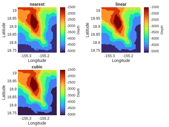
Interpolation Modes in Practice

Nearest

• Fastest local interpolation rule.
• Most blocky output.
• Useful as a coarse baseline and for sanity checks.
• Rarely, rarely used in practice for final output because it can miss important local trends and create artificial discontinuities.

Linear

• Usually the best default for reliability and speed-quality balance.
• Piecewise-linear local behavior often avoids overshoot artifacts.
• Good starting point for engineering lookup tables.
• Extremum are always at grid points, which can be desirable for some applications.
• It’s the most consistent with the regularization meaning a true linear underlying function has no regularization penalty.

Cubic

• Smoother local appearance and gradients.
• Wider local stencil increases coupling and can increase runtime.
• More sensitive to sparse/noisy regions; use only when you need smoother local derivatives.
• Extremum can be between grid points, which can be desirable for some applications but also can lead to overshoot artifacts.

Interpolation Comparison Run

Use one fixed dataset and only change interpolation mode to see differences. The timing difference do not approach their asymptotic complexity differences because the problem size is small, but you should see some difference in output shape.

clc; clear; close all;

data = load('a01_etopo_loihi.mat');
x = double(data.x);
y = double(data.y);
z = double(data.z);

xLimits = [min(x), max(x)];
yLimits = [min(y), max(y)];

xGrid = {linspace(xLimits(1), xLimits(2), 50), ...
         linspace(yLimits(1), yLimits(2), 51)};

smoothness = 1e-4;
modes = {'nearest', 'linear', 'cubic'};


tiledlayout(2,2, 'Padding', 'compact', 'TileSpacing', 'compact')

for k = 1:numel(modes)
  tic;
    zGrid = regularizeNd([x,y], z, xGrid, smoothness, modes{k});
  zFunction = griddedInterpolant(xGrid, zGrid, modes{k});
    t = toc;
    fprintf('%-7s runtime: %.3f s\n', modes{k}, t);
    nexttile
  fcontour(@(x,y) reshape(zFunction(x(:),y(:)), size(x)), [xLimits, yLimits],"Fill","on")
    axis tight
    title(modes{k})
    xlabel('Longitude')
    ylabel('Latitude')
    colormap(turbo)
    cb = colorbar;
    cb.Label.String = 'Depth';
end

nearest runtime: 0.087 s
linear  runtime: 0.025 s
cubic   runtime: 0.041 s

What to inspect:

• local roughness around sparse regions,
• edge behavior near low-sample zones,
• whether visually smooth output still respects major trend features.

Solvers

regularizeNd supports multiple solve pathways. For this project, a practical policy is:

1. Try normal first for speed.
2. If warnings or conditioning issues appear, switch to \ for robustness.
3. Use iterative solvers when memory or factorization cost becomes limiting.

Solver Comparison Run

Keep interpolation and grid fixed. Compare solver choices on the same matrix build.

clc

data = load('a01_etopo_loihi.mat');
x = double(data.x);
y = double(data.y);
z = double(data.z);

xLimits = [min(x), max(x)];
yLimits = [min(y), max(y)];

xGrid = {linspace(xLimits(1), xLimits(2), 500), ...
         linspace(yLimits(1), yLimits(2), 501)};

smoothness = 1e-4;
interpMethod = 'linear';

solverList = ["normal", "\", "pcg", "symmlq", "lsqr"];
maxIterations = 4e4;
solverTolerance = 1e-8;

for i = 1:numel(solverList)
    solver = solverList(i);

    tic
    if any(solver == ["pcg", "symmlq", "lsqr"])
        zGrid = regularizeNd([x,y], z, xGrid, smoothness, interpMethod, solver, maxIterations, solverTolerance);
    else
        zGrid = regularizeNd([x,y], z, xGrid, smoothness, interpMethod, solver);
    end
    t = toc;

    fprintf('%-7s runtime: %.3f s\n', char(solver), t);

    if any(~isfinite(zGrid), 'all')
        warning('Non-finite values detected with solver %s', char(solver));
    end
end

normal  runtime: 1.146 s
\       runtime: 2.885 s
pcg     runtime: 13.404 s
symmlq  runtime: 12.943 s
lsqr    runtime: 64.713 s

Decision Rules

Start here, then refine:

1. Use linear interpolation and smoothness = 1e-4 as a neutral baseline for this dataset. 1e-3 is the most common starting point across most datasets. This data set contains a lot of data and therefore can use smaller smoothness relying on the local high fidelity data to control the fit. If you have less data, you may need more smoothness to get a good fit.
2. Try normal first when no rank/conditioning warnings appear (99.9% of the time). Lowering the smoothness far enough will trigger warnings, which is a sign to switch to \ for robustness.
3. Switch to \ when robustness is more important than speed.
4. Switch to iterative pathways when matrix size pushes memory or direct-factorization cost too high. For this dataset, the direct solvers are fast and the iterative solvers are slow. The problem size is not yet large enough that the iterative solvers are competitive, but this will change as you increase the grid size.

Common Failure Modes

1. Overfitting appears as local wiggles despite visually smooth broad trend.
2. Ill-conditioning appears as unstable runtimes, warnings, or wildly different fits from small option changes.
3. Solver mismatch appears as long runtime with no quality gain.

Checklist Before Moving On

1. You recorded at least one solver runtime sweep on the same data/grid.
2. You compared the results across the different solvers.

Key Point

Interpolation choice should be based on output behavior and accuracy needs, not only local computational complexity.

Next

Part 4: Boundary Behavior and Convex Hull