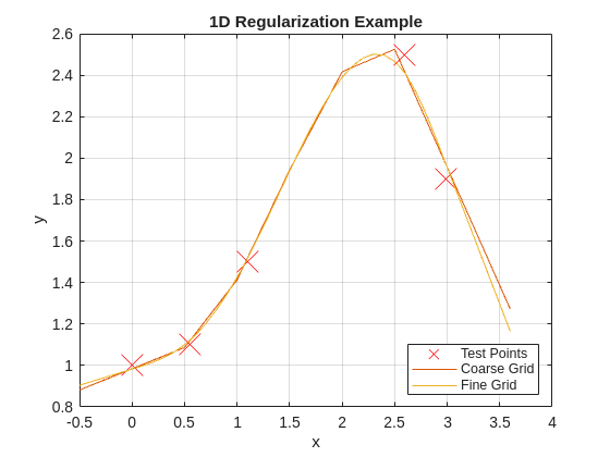
The script uses a small 1D dataset from the original Math for Mere Mortals educational blog progression and compares coarse and fine grids under the same smoothness value.
Why 1D First
In higher dimensions, you may not immediately distinguish noise tracking from true structure. In 1D, the failure modes are visually obvious, so you can establish parameter discipline before moving to 2D and nD cases.
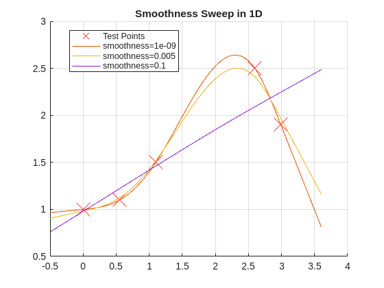
smoothnessList= [1e-9,5e-3,1e-1];figure;holdon;gridon;plot(x,y,'rx','MarkerSize',20,'DisplayName','Test Points')fork=1:numel(smoothnessList)s=smoothnessList(k);yGrid=regularizeNd(x,y,xGridFine,s);plot(xGridFine{1},yGrid,'DisplayName',sprintf('smoothness=%g',s));endlegend('show','location','best');title('Smoothness Sweep in 1D');
The example comments note that extremely tiny values can make the system ill-conditioned, which is exactly why log-step sweeps are better than random tweaking.
Interpretation Rules
If curve oscillations appear between sparse data points, smoothness is likely too low.
If the curve misses clear trend changes, smoothness is likely too high.
If coarse and fine grids tell opposite stories, treat that as a warning and retune.
Repeatable Tuning Workflow
Start at 1e-2 or 5e-3.
Move by factors of 10 only.
Lock a candidate value where trend fidelity and smoothness are both acceptable.
Validate with at least one alternate grid density.
Common Mistakes
Changing smoothness, interpolation, and solver all at once.
Using linear-scale sweeps such as 0.001, 0.002, 0.003 before understanding order-of-magnitude behavior. Use linear scaling after you have a good candidate value to fine-tune around.
Ignoring conditioning warnings at tiny smoothness values.
Next Step
Proceed to Part 3 to evaluate interpolation method and solver behavior using the parameter discipline built here.