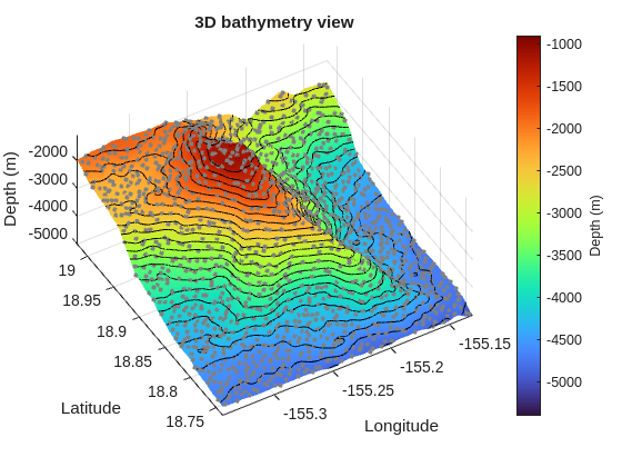
This script uses a01_etopo_loihi.mat, a local subset derived from NOAA ETOPO 2022 (NOAA National Centers for Environmental Information 2022), centered on Kamaʻehuakanaloa Seamount. It defines a 2D grid, solves for a gridded surface with regularizeNd, upsamples the fitted surface for visualization, and compares scattered data against the fitted surface.
regularizeNd solves a sparse least-squares problem that combines:
fidelity equations from interpolating the scattered data
smoothness equations from regularization operators
In plain terms:
lower smoothness gives tighter tracking of noisy points
higher smoothness gives more stable and cleaner surfaces
The right value depends on measurement noise, expected physics, and how much local detail you need to preserve.
Minimal Reproducible Run
clc;clear;closeall;data=load('a01_etopo_loihi.mat');x=double(data.x);y=double(data.y);z=double(data.z);xLimits= [min(x),max(x)];yLimits= [min(y),max(y)];xGrid= {linspace(xLimits(1) -eps(xLimits(1)),xLimits(2) +eps(xLimits(2)),480),...linspace(yLimits(1) -eps(yLimits(1)),yLimits(2) +eps(yLimits(2)),481)};smoothness=0.000001;zGrid=regularizeNd([x,y],z,xGrid,smoothness,'cubic');% equivalents ways to call regularizeNd% zGrid = regularizeNd([x,y], z, xGrid, smoothness, 'cubic', 'normal');% Upsample grid since we are using cubic interpolationzFunction=griddedInterpolant(xGrid,zGrid);xGrid2= {linspace(xLimits(1) -eps(xLimits(1)),xLimits(2) +eps(xLimits(2)),2000),...linspace(yLimits(1) -eps(yLimits(1)),yLimits(2) +eps(yLimits(2)),2001)};xGrid2Expanded=cell(2,1);[xGrid2Expanded{:}] =ndgrid(xGrid2{:});zGrid2=zFunction(xGrid2Expanded{1},xGrid2Expanded{2});surf(xGrid2{:},zGrid2','EdgeColor','none','FaceColor','interp')holdon;contour3(xGrid2{:},zGrid2',22,'k','LineWidth',0.45)GRAY= [0.50.50.5];scatter3(x,y,z,10,GRAY,'filled')colormap(turbo(256))clim([-5400-900])view(329.7,61)xlabel('Longitude')ylabel('Latitude')zlabel('Depth (m)')gridonaxistighttitle('3D bathymetry view')ylabel(colorbar,'Depth (m)')
What To Change First
Keep the same grid and vary smoothness across orders of magnitude.
Compare surface roughness and local peaks.
Keep interpolation fixed initially so you isolate smoothness effects.
Suggested quick sweep values:
1e-6
1e-4
1e-2
The example dataset is intentionally undersampled, so use this first pass to tune smoothness expectations rather than to recover every local summit detail.
How To Read The Plot
Look for three common regimes:
Too low smoothness: the fitted surface chases local noise.
Balanced smoothness: broad trend and local structure are both visible.
Too high smoothness: physically meaningful gradient changes are flattened and the surface becomes too linear in each axis.
Practical Notes
If your data is sparse near boundaries, expect extrapolation behavior to reflect regularization assumptions more strongly than fidelity.
If one axis is rougher than another, use per-axis smoothness strategy instead of forcing one global value.
Keep this first pass simple: tune smoothness before exploring solver and interpolation alternatives.
Next Step
Continue to Part 2 to isolate parameter behavior in 1D and build a reproducible smoothness tuning workflow.
NOAA National Centers for Environmental Information. 2022. “ETOPO 2022 15 Arc-Second Global Relief Model.” NOAA National Centers for Environmental Information. https://doi.org/10.25921/fd45-gt74.