In simulation and controls, its important to understand the details of a second order system. This post is how the damping ratio affect the poles of a second order system.
The mechanical second order system has the following form:
\[m \ddot{x} + c \dot{x} + k x = F(t)\]
Where:
- \(m\) is the mass
- \(c\) is the damping coefficient
- \(k\) is the spring constant
- \(F(t)\) is the external force applied to the system
Normalizing the equation by dividing through by \(m\) gives:
\[\ddot{x} + 2 \zeta \omega_n \dot{x} + \omega_n^2 x = \frac{1}{m}F(t)\]
Where:
- \(\omega_n = \sqrt{\frac{k}{m}}\) is the natural frequency
- \(\zeta = \frac{c}{2 \sqrt{mk}}\) is the damping ratio
Taking the laplace transform with 0 initial conditions gives the transfer function. Note, that the 0 initial conditions can be handled later and that studying the damping ratio effects on the poles is independent of initial conditions.
\[G(s) = \frac{X(s)}{F(s)} = \frac{\frac{1}{m}}{s^2 + 2 \zeta \omega_n s + \omega_n^2}\]
The poles of this system represent the roots of the denominator and can be found using the quadratic formula:
\[s = \frac{-2 \zeta \omega_n \pm \sqrt{(2 \zeta \omega_n)^2 - 4 \cdot 1 \cdot \omega_n^2}}{2 \cdot 1}\]
Let’s normalize this expression by dividing through by \(\omega_n\) and simplify the expression:
\[\frac{s}{\omega_n} = -\zeta \pm \sqrt{\zeta^2 - 1}\]
What’s important is understanding how the damping ratio \(\zeta\) affects the nature of the poles.
- No damping (\(\zeta = 0\)):
- The poles are purely imaginary: \(s = \pm j \omega_n\).
- This indicates undamped oscillations at the natural frequency \(\omega_n\).
- Underdamped (\(0 < \zeta < 1\)):
- The poles are complex conjugates: \(s = -\zeta \omega_n \pm j \omega_n \sqrt{1 - \zeta^2}\).
- This indicates oscillatory behavior with an exponential decay determined by the real part \(-\zeta \omega_n\).
- Critically damped (\(\zeta = 1\)):
- The poles are real and repeated: \(s = -\omega_n\).
- This indicates the system returns to equilibrium as quickly as possible without oscillating.
- Overdamped (\(\zeta > 1\)):
- The poles are real and distinct: \(s = -\zeta \omega_n \pm \omega_n \sqrt{\zeta^2 - 1}\).
- This indicates a non-oscillatory return to equilibrium, with the speed of return depending primarily on the larger of the two poles.
- As the damping ratio goes to infinity, one pole approaches zero while the other goes to negative infinity.
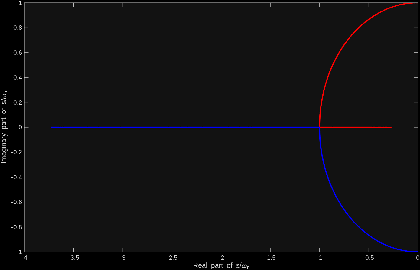
Below is a plot of the poles of a second order system as a function of the damping ratio from 0 to 2. Note how when the poles become real, one pole goes to zero while the other goes to negative infinity as the damping ratio increases.
zeta = unique([linspace(0,1,1001), linspace(1,2,100)]).';
rootWithPositiveImaginaryPart = -zeta + sqrt(zeta.^2 -1);
rootWithNegativeImaginaryPart = -zeta - sqrt(zeta.^2 -1);
plot(rootWithPositiveImaginaryPart, 'r', 'LineWidth', 2);
hold on;
axis equal;
plot(rootWithNegativeImaginaryPart, 'b', 'LineWidth', 2);
xlabel('Real part of s/\omega_n');
ylabel('Imaginary part of s/\omega_n');