This part documents the historical lineage of regularizeNd and gives practical migration guidance for users coming from gridfit or RegularizeData3D.
Practical Goal
How regularizeNd relates to earlier tools.
Map common gridfit and RegularizeData3D patterns to regularizeNd equivalents.
Example Anchor
Primary migration examples in this part: regularizeNd/Examples/From gridfit/demo_from_gridfit.m rewrite and regularizeNd/Examples/From RegularizeData3D rewrite patterns.
regularizeNd is inspired by earlier regularized surface fitting tools in the MATLAB ecosystem. Two tools are particularly relevant as a conceptual starting point:
gridfit (John D’Errico) (D’Errico 2016) — a 2-D input surface fitting tool using a similar regularization philosophy. gridfit introduced many users to the idea of balancing data fidelity against smoothness on a grid.
RegularizeData3D(Jamal 2014) — extended the concept to cubic interpolation. Made the smoothness parameter reusable across problems by scaling the regularization relative to the fidelity term.
regularizeNd generalizes the approach to an arbitrary number of input dimensions, fixed some all zero rows in gridfit and RegularizeData3D,exposes the underlying matrices for constrained problems, and provides multiple solver options including iterative solvers for large systems.
Important framing: regularizeNd is inspired by this prior work and shares the regularization concept, but it is an independent implementation.
Migrating from gridfit
Conceptual mapping
gridfit concept
regularizeNd equivalent
gx, gy (grid vectors)
xGrid = {gx, gy}
'smoothness' property (default 1), scalar, vector
smoothness positional arg (similar role, different scaling/defaults), scalar, vector
regularizeNd’s regularization is fixed to the gradient regularizer because the others don’t work well.
Output is in meshgrid format
Output is in ndgrid format — transpose before plotting with surf
Minimal gridfit → regularizeNd rewrite
% --- gridfit (old) ---% g = gridfit(x, y, z, gx, gy, smoothness);% surf(gx, gy, g) % gridfit output is meshgrid-formatted% --- regularizeNd (new) ---g=regularizeNd([x,y],z, {gx,gy},smoothness);surf(gx,gy,g') % note the transpose: regularizeNd output is ndgrid-formatted
The transpose g' is the most common source of confusion. regularizeNd stores the output in ndgrid format (g(i,j) indexes gx(i), gy(j)), while MATLAB’s surf expects meshgrid format (g(j,i)).
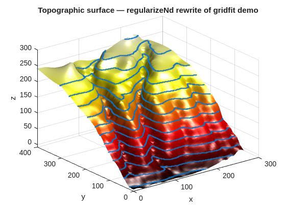
Topographic data demo rewrite
Below is the first section of demo_from_gridfit.m rewritten in clean regularizeNd style. The original used bluff_data.mat (Two ravines on a hillside, scanned from a topographic map of upstate New York).
clc;clear;closeall;loadbluff_datax=bluff_data(:,1);y=bluff_data(:,2);z=bluff_data(:,3);gx=0:4:264;gy=0:4:400;smoothness=1e-5;g=regularizeNd([x,y],z, {gx,gy},smoothness);figurecolormap(hot(256))surf(gx,gy,g') % transpose for surfcamlightright;lightingphong;shadinginterpline(x,y,z,'Marker','.','MarkerSize',4,'LineStyle','none')title('Topographic surface — regularizeNd rewrite of gridfit demo')xlabel('x');ylabel('y');zlabel('z')
% --- RegularizeData3D (old) ---% g = RegularizeData3D(x, y, z, xnodes, ynodes, ...% 'smoothness', smoothness, 'interp', 'bicubic');% --- regularizeNd (new) ---g=regularizeNd([x,y],z, {xnodes,ynodes},smoothness,'cubic');% same ndgrid output format — surf(xnodes, ynodes, g') for display
The key structural change is that the separate x, y scatter inputs become the two columns of a single matrix argument.
Interpolation naming is not one-to-one: in practice, RegularizeData3D'bicubic' aligns with regularizeNd'cubic', and RegularizeData3D'bilinear' align most closely with regularizeNd'linear'.
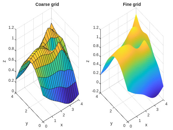
Coarse vs. fine grid demo rewrite
This example is adapted from From RegularizeData3D/coarse_vs_fine_grids.m and demonstrates a key property: for the same smoothness value, the fitted surface is nearly identical regardless of grid resolution. Coarser grids are faster; finer grids give more evaluation points.
Both panels should show essentially the same surface shape. The fine grid has more evaluation resolution, not a fundamentally different result.
What regularizeNd Does Not Do
To be precise about scope:
It does not guarantee interpolation through every data point — it is a weighted least-squares fit. Use smoothness → 0 if you want near-interpolation behavior (at the cost of the smoother no longer regularizing effectively).
It does not enforce physical constraints automatically. Use regularizeNdMatrices + lsqlin or lsqConstrainedAlternative for that (see Part 6).
It does not currently support unstructured output grids. The output is always on a rectilinear ndgrid.
Quick Reference: Common Output Format Confusion
regularizeNd outputs in ndgrid format. Most MATLAB visualization functions expect meshgrid format. The relationship is:
% regularizeNd output: zGrid(i,j) ↔ xGrid{1}(i), xGrid{2}(j)% surf/mesh/contourf expect: Z(j,i) for plotting against x, y vectorssurf(xGrid{1},xGrid{2},zGrid') % 2-D case: transpose zGrid
For 3-D and higher, use permute or griddedInterpolant to handle the indexing convention explicitly.