This article is the rigorous companion to the tutorial series. It documents how regularizeNd constructs and solves its optimization problem, then shows how to generalize the regularizer operator by axis and derivative order.
Attribution and Lineage
The educational progression is inspired by Peter Goldstein’s regularization articles and related historical tools D’Errico (2016)Jamal (2014). The implementation discussed here is regularizeNd and this article is independently written for that codebase.
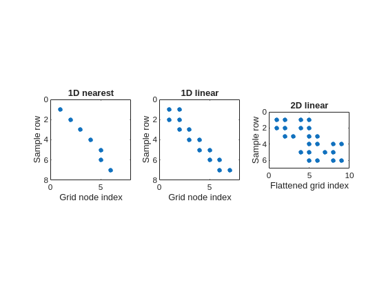
These two examples show the row structure explicitly. The next examples show the full sparse-pattern structure of the fidelity matrix.
Example C: spy plots of fidelity matrices
The easiest way to see the global structure of \(A_f\) is with sparse-pattern plots. In regularizeNd, each interpolation mode changes the number and arrangement of nonzeros per row.
nearest interpolation gives exactly one nonzero per row,
1D linear interpolation gives exactly two neighboring nonzeros per row,
2D linear interpolation gives exactly four nonzeros per row, but those four entries are separated in the flattened indexing because the 2D grid has been unwrapped into one column vector.
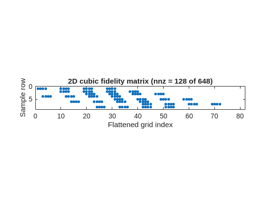
Example D: cubic fidelity patterns are wider
Higher-order interpolation widens the fidelity row stencil. In 2D cubic interpolation, each row touches \(4^2=16\) nearby grid values.
That is the same fidelity concept as the earlier algebraic examples, just viewed as a whole sparse matrix instead of one row at a time.
nD Lookup Table Unwrapping and Linear Indexing
regularizeNd uses MATLAB linear indexing to represent an nD lookup table as a vector of unknowns.
Let grid size be \((n_1,\dots,n_d)\) and total unknowns \(N=\prod_{m=1}^d n_m\). The unknown table \(Z\in\mathbb{R}^{n_1\times\cdots\times n_d}\) is vectorized as \(z\in\mathbb{R}^{N}\).
For subscript \((i_1,\dots,i_d)\), MATLAB-style 1-based linear index is:
Here \(\operatorname{ind}\) is just a name for the linear-index mapping. It means “the vector position corresponding to subscripts \((i_1,\dots,i_d)\)”. It is not special MATLAB syntax; it is only a label for the indexing formula.
This is exactly why fidelity and smoothness stencils become sparse rows in a single global linear system. It avoids treating each axis separately in custom tensor solvers and keeps the assembly compatible with MATLAB sparse operators.
Graphical 3D unwrapping example: array size [3 4 5]
Suppose
\[
Z = \operatorname{reshape}(1:60,[3,4,5]).
\]
Then MATLAB fills the first dimension first. The five slices are:
This is the concrete mechanism regularizeNd relies on when it assembles nD interpolation and regularization stencils into one sparse linear system.
Regularization
Regularization blocks
For each axis, regularizeNdMatrices builds a sparse block \(L_k\) based on second-derivative finite-difference stencils. For non-uniform grids, weights are computed from local spacing, not a uniform-grid assumption.
Per axis, each regularization row has three nonzero entries tied to adjacent grid nodes along that axis.
For axis coordinate triplet \((x_{i-1},x_i,x_{i+1})\) and unknown samples \((z_{i-1},z_i,z_{i+1})\), the second-derivative stencil used in code is:
fidelity rows pull the solution toward measured scattered data,
smoothness rows pull the solution toward smoothly varying gradients.
The practical tradeoff is controlled by the scaled magnitude of each \(L_k\) relative to \(A_f\).
How to interpret the smoothness value
In regularizeNd usage, smoothness is best interpreted as the approximate ratio of smoothness importance to fidelity importance after the built-in normalization and axis scaling are applied.
So, as a tuning rule of thumb:
\(s=1\) means smoothness and fidelity are treated as comparably important,
\(s=10^{-3}\) means smoothness is treated as roughly \(1/1000\) as important as fidelity,
smaller values push the fit toward the data more aggressively,
larger values push the fit toward smoother directional gradients.
That interpretation is exactly why the project documentation describes smoothness as the ratio of smoothness to goodness of fit.
Why smoothness-count normalization matters
Without normalization, changing grid density changes how many smoothness equations are present, which would implicitly retune smoothness even when user intent is unchanged.
Using \(\sqrt{N_f/N_{s,k}}\) normalizes for number fidelity equations versus smoothness equations from each axis. Smoothness values generalize and not problem and grid-specific.
Why range scaling matters
If one axis spans values like \(10^{-3}\) and another spans \(10^3\), raw derivatives are numerically imbalanced. Multiplying by \((x_{k,\max}-x_{k,\min})^2\) is equivalent to derivative scaling under normalization to a unit axis, reducing this magnitude bias.
So the regularizer behaves more consistently when axes have drastically different magnitudes.
Smoothness transferability across similar problems
Because of smoothness-count and axis-range normalization, a chosen smoothness value is often reusable across similar datasets and grids in regularizeNd. This is a practical difference from older workflows such as gridfit, where retuning is more sensitive to grid and scale changes.
Exact Zero-Penalty Function Class
The most useful structural fact is the null space of the regularizer. If the second derivative along every axis is exactly zero, then the function is linear in each axis.
That means:
in 1D, the exact zero-penalty class is affine,
in 2D, it is bilinear,
in 3D, it is trilinear,
in nD, it is multilinear.
The same nD pattern can be written in more familiar expanded notation as
When expanded, this produces a constant term, every single-axis term, every pairwise product, every triple product, and so on up to the full product of all axes. Each variable appears with power at most 1, so every pure second derivative with respect to a single axis vanishes.
More generally, the full multilinear null-space class is any linear combination of those expanded terms. The product form above is the most compact way to picture why the regularizer is exactly satisfied by functions that are linear in each coordinate separately.
This is a better mental model than treating the regularizer as a generic smoothing penalty. The operator is really expressing a preference for grid functions whose directional gradients vary slowly, with exact agreement when the table is multilinear.
Solving
Solve stage
regularizeNd concatenates rows into
\[
A = \begin{bmatrix}A_f\\L_1\\\vdots\\L_n\end{bmatrix},\qquad
b = \begin{bmatrix}y\\0\\\vdots\\0\end{bmatrix}
\]
and solves with one of the configured pathways:
direct backslash on \(A\)
normal equations on \(A^TA\)
iterative pathways (pcg, symmlq, lsqr), including preconditioning support
Why the Normal Solver Is Often Faster
For this sparse least-squares form, constructing and solving normal equations
\[
(A^TA)z=A^Tb
\]
is typically much faster in regularizeNd tests for large grids. The project notes report about 3x speedup versus direct sparse backslash, and the direct project guidance is to try normal first on well-conditioned problems.
Key reason: sparse structure is preserved well enough that factorization cost is often lower than solving rectangular sparse least squares directly.
In practice:
normal-equation solve is commonly handled by sparse Cholesky factorization of symmetric positive-definite systems,
direct sparse backslash on rectangular \(A\) is generally based on sparse QR.
For regularizeNd-style systems, this normal-equation route is practical to large systems. A useful rule of thumb from project experience is that roughly \(2\times 10^6\) grid points can still be solved on a normal 32 GB laptop in about 10 to 60 seconds when the problem is well-conditioned and the sparsity pattern remains favorable.
Sparse QR remains the safer default when ill-conditioning is a concern, for example very small smoothness values with small amount data and large number of grid points.
So recommended policy is:
try normal first for speed on well-conditioned problems,
use direct sparse QR when rank/conditioning warnings appear,
above roughly the \(2\times 10^6\) grid point scale, or whenever memory becomes the practical limit, switch to iterative pathways.
For iterative order, the project guidance is:
start with pcg,
then try symmlq,
finally use lsqr as a last resort.
That ordering mirrors the example notes: pcg and symmlq are usually much faster than lsqr, while lsqr remains valuable when the normal-equation iterative methods struggle.
Why Incomplete Cholesky Is the Default General Preconditioner
The iterative pcg and symmlq paths solve the normal equation
\[
(A^TA)z = A^Tb,
\]
so the coefficient matrix is symmetric and, in the regularized full-rank case, positive definite. That is exactly the setting where incomplete Cholesky is the natural general-purpose preconditioner.
regularizeNd therefore uses incomplete Cholesky when possible, with diagonal compensation fallback when needed. This is a strong default because it matches the algebraic structure of the matrix being solved rather than treating the system as a generic nonsymmetric least-squares problem.
Why Second Derivative Is the Current Default
A second-derivative penalty suppresses rapid changes in gradient. In sparse-data regions, this tends to produce behavior that is linear in each axis, which is often desirable for stable interpolation and pragmatic extrapolation behavior.
Conceptually, this corresponds to discouraging large values of \(\partial^2 f / \partial x_k^2\) for each axis.
so penalizing second derivative is penalizing rapid variation of slope. In other words, it promotes smooth gradients, not necessarily flat gradients.
This is why the method can keep broad trends while damping jagged high-frequency behavior.
Extension
Mapped-Coordinate Extension
Another useful extension is to change coordinates before fitting. This is the core idea behind the mapping workflow in Part 6 and in constraint_and_Mapping_Example.m.
Suppose the original independent variable \(x\) produces a difficult relationship, but a monotone transformed coordinate
\[
u = g(x)
\]
makes the surface smoother. Then solve for the lookup table in \(u\) rather than directly in \(x\):
After solving, evaluation is just composition: map the query point into the transformed coordinate and interpolate there.
The advantage is not only that the fitted table can become smoother. It also makes many dual or inverse formulations much easier:
if the forward map is sharp or badly scaled, a transformed forward coordinate may become closer to multilinear,
if an inverse map is smoother and monotone, fit the inverse table directly instead of forcing the rougher forward map,
if a log, semilog, or custom monotone warp straightens one axis, the same sparse least-squares machinery still applies with no conceptual change to the solver.
This is powerful because regularizeNd operates on table values after discretization. Once the coordinates are mapped, the fidelity and regularization machinery is unchanged. You have effectively changed the problem geometry without changing the optimization backbone.
In practice, that means the same matrix-assembly pattern can support:
smoother forward lookup tables,
inverse lookup tables when the inverse problem is better conditioned,
dual formulations where a physically awkward variable is replaced by a more regular latent coordinate.
That flexibility is one of the strongest practical arguments for a lookup-table formulation: coordinate design, regularizer design, and constraint design can all be modified while keeping the core sparse least-squares solve recognizable.
Constrained Least-Squares Extension
Another important extension is constraint handling. Because regularizeNd already builds a sparse linear least-squares problem in the lookup-table values themselves, adding many useful constraints is straightforward.
The unconstrained stacked system is
\[
\min_z \|Az-b\|_2^2.
\]
Linear constraints extend this naturally to
\[
\min_z \|Az-b\|_2^2
\quad\text{subject to}\quad
C_{eq}z=d_{eq},\qquad Cz\le d.
\]
This is attractive because the unknowns are grid values, not parameters of a nonlinear symbolic model. The underlying physical relationship may be nonlinear, but once it is discretized onto the grid, many desired behaviors become linear equalities or inequalities in the unknown table entries.
Examples that discretize cleanly include:
monotonicity constraints,
upper and lower bounds on the table values,
bounded slope constraints,
convexity or concavity constraints via finite differences,
region-specific tie constraints or anchor conditions.
In other words, the function represented by the table can be nonlinear in the physical variables while the optimization over table entries remains a convex constrained least-squares problem.
That is a major practical advantage of the lookup-table formulation: global solutions are still easy to compute even when the modeled relationship itself is nonlinear.
Why this works well in regularizeNd
The matrix structure is already sparse and local:
fidelity rows only touch nearby interpolation nodes,
smoothness rows only touch local stencil nodes,
many useful constraints also only touch local neighboring nodes.
So the constrained problem preserves the same sparse-operator flavor as the unconstrained one.
The current codebase already reflects this extension path through monotonicConstraint.m and lsqConstrainedAlternative.m.
Discretized nonlinear constraints
Even some constraints that are nonlinear when stated on a continuous function become easy to encode after discretization.
For example, statements like
“the table should be monotone increasing in flow”,
“the slope should stay nonnegative in this operating region”,
“the curvature sign should not change here”,
can be enforced using finite-difference relations on neighboring grid entries. Once written in those discrete variables, the solve often remains linear or convex.
That means one can incorporate substantial physical structure without giving up the ability to compute a global optimum reliably.
Third-Order Regularization Extension
This section is intentionally isolated as an extension concept, not a required default path.
When a Third Derivative Is More Appropriate
If one axis is expected to be near-parabolic across the operating region, second-derivative penalization can over-flatten physically meaningful gradient change or require a larger number of grid points. In that case, penalizing the third derivative along that axis can be a better structural prior.
Typical engineering pattern: pressure-flow-position couplings where one direction exhibits approximately quadratic trends over relevant operating windows. i.e. Pressure as the output and flow as input axis, using a third-derivative penalty implies a parabolic relationship between pressure flow implicitly encoded in the regularizer and thus extrapolation behavior encodes the expected parabolic trend.
Penalizing third derivative encourages piecewise-quadratic behavior by discouraging rapid changes of second derivative. Equivalently, it allows gradients to vary approximately linearly instead of forcing each axis toward multilinear behavior.
Swapping the Regularizer Operator
The regularizer should be treated as an operator design choice. A practical mixed-order objective is
with \(S_2\cup S_3=\{1,\dots,n\}\) and \(S_2\cap S_3=\emptyset\).
Interpretation:
axes in \(S_2\): linear-trend prior in sparse regions
axes in \(S_3\): quadratic-trend prior in sparse regions
Numerical Implications of Third Derivative Blocks
Expected impacts when moving from order 2 to order 3 on selected axes:
stronger sensitivity to local spacing quality along that axis
potential condition-number increase in the assembled normal matrix
greater need for preconditioning quality checks in iterative solves
higher risk of oscillatory behavior if data are sparse and weight is too small
These are manageable if derivative order is used selectively and validated against physical priors.
Practical Selection Rule: Second vs Third Derivative
Use second derivative on an axis when:
local linear continuation is plausible in sparse zones
monotonic or gently varying behavior dominates
Use third derivative on an axis when:
local quadratic structure is expected from physics or mechanism
preserving linearly changing gradients is important for prediction quality
Use mixed order when:
different axes have different expected structure
one axis is near-parabolic while others are not
Validation Protocol for Mixed-Order Design
Hold scattered data, grid, and interpolation method fixed.
Compare operator maps: all-second vs mixed-order candidate sets.
Report:
train residual norm
physically relevant slice behavior
edge and extrapolation behavior near sparse boundaries
solver convergence statistics and runtime
Select the lowest-complexity operator map that meets physical plausibility and prediction error targets.
Limits and Scope
This article describes a mathematically and computationally consistent extension pathway. It does not claim that mixed-order regularization is always better. The benefit depends on whether derivative-order priors match the underlying system.
Implementation Path for regularizeNd
This section outlines a direct extension strategy without changing the external conceptual model.
Extend operator construction in regularizeNdMatrices:
add derivative-order control per axis, for example an integer vector with values 2 or 3
keep scalar-to-vector expansion behavior consistent with current smoothness handling
Add third-derivative stencil generator:
keep existing secondDerivativeWeights for order 2
add thirdDerivativeWeights for order 3 on non-uniform grids
require minimum grid points per axis based on derivative order (order 3 requires at least 4 points)
Generalize row indexing logic:
current second-derivative blocks use 3-point stencils and 3 column indices per row
third-derivative blocks will use 4-point stencils and 4 column indices per row
compute equation counts per axis as \(n_k-\text{order}\) rather than hard-coded \(n_k-2\)
Preserve scaling policy:
retain smoothness-equation normalization and axis scaling for both derivative orders
tune separate per-axis weights when combining orders, because operator magnitudes differ
Keep solver interface unchanged initially:
output remains stacked sparse least-squares system
existing direct and iterative solve paths remain valid
Variables and Notation
This section defines symbols used across the fidelity, regularization, solving, and extension equations.
Core Unknowns and Data
\(z\): vectorized lookup-table unknowns (all grid values stacked into one column vector).
\(Z\): nD lookup table before vectorization.
\(y\): measured scattered-data values used by the fidelity equations.
\(x\): original independent variable (or coordinate vector) in mapped-coordinate discussions.
\(u = g(x)\): mapped coordinate after monotone transformation.