Trapezoidal Rule for Numerical Integration
Source inspiration: (Mathew 2000-2019).
Description
The composite trapezoidal rule approximates \(\int_a^b f(x)\,dx\) by replacing \(f\) on each subinterval with a line segment between neighboring nodes. Summing the trapezoid areas gives \[ T_n = h\left[\tfrac12 f(x_0) + \sum_{i=1}^{n-1} f(x_i) + \tfrac12 f(x_n)\right], \quad h=\frac{b-a}{n}. \]
For smooth functions, the global truncation error is second order: \(T_n - I = O(h^2)\). Geometrically, accuracy improves as node spacing is reduced across the full interval.
Animations
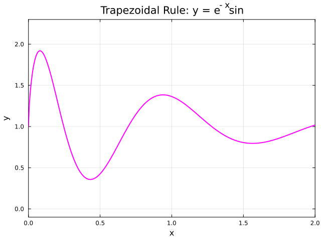
Each animation below shows the trapezoidal rule diagram over \([0,2]\) for \(y = e^{-x}\sin(8x^{2/3})+1\). Each new frame recomputes the approximation on the full interval with a denser partition.
Julia source scripts that generated these animations are linked under each case.
Case 1 — Composite Trapezoidal Rule, \(f(x)=e^{-x}\sin(8x^{2/3})+1\) on \([0,2]\)
Behavior: As the number of sample points increases, trapezoids across the entire interval become narrower, and the approximation converges toward the true integral with \(O(h^2)\) global error.
Derivation Notes (Planned)
Short derivations will be added to explain the core equations and assumptions.
Worked Example (Planned)
A compact numerical example with intermediate steps will be included.
Implementation Notes (Planned)
Implementation details, numerical stability notes, and practical pitfalls will be added.