Simpson’s Rule for Numerical Integration
Source inspiration: (Mathew 2000-2019).
Description
Composite Simpson’s rule approximates \(\int_a^b f(x)\,dx\) by fitting a quadratic interpolant across each pair of subintervals. With \(h=(b-a)/n\) and even \(n\), \[ S_n = \frac{h}{3}\left[f(x_0)+f(x_n)+4\sum_{k=1}^{n/2} f(x_{2k-1}) + 2\sum_{k=1}^{n/2-1} f(x_{2k})\right]. \]
Because the method integrates cubics exactly, the composite error for smooth functions is \(O(h^4)\), typically much smaller than trapezoidal error at the same spacing.
Animations
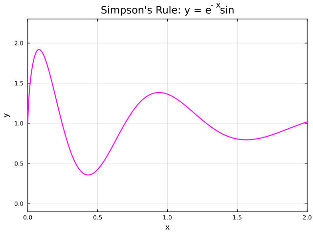
Each animation below shows the Simpson’s rule diagram over \([0,2]\) for \(y = e^{-x}\sin(8x^{2/3})+1\). Each frame redraws the entire interval using a denser even partition.
Julia source scripts that generated these animations are linked under each case.
Case 1 — Composite Simpson’s Rule, \(f(x)=e^{-x}\sin(8x^{2/3})+1\) on \([0,2]\)
Behavior: Quadratic panels are rebuilt over the full interval as sample density increases, and the approximation converges rapidly with fourth-order global accuracy.
Derivation Notes (Planned)
Short derivations will be added to explain the core equations and assumptions.
Worked Example (Planned)
A compact numerical example with intermediate steps will be included.
Implementation Notes (Planned)
Implementation details, numerical stability notes, and practical pitfalls will be added.