Newton Interpolation Polynomial
Source inspiration: (Mathew 2000-2019).
Description
Newton interpolation represents the interpolating polynomial in divided-difference form,
\[ P_n(x)=a_0 + a_1(x-x_0)+a_2(x-x_0)(x-x_1)+\cdots+a_n\prod_{j=0}^{n-1}(x-x_j), \]
where \(a_k=f[x_0,\ldots,x_k]\) are divided differences. For the same nodes and data, Newton and Lagrange forms produce the same polynomial; they differ only in representation and numerical workflow.
The 29 animations below intentionally reuse the same interpolation cases as the Lagrange page, matching the legacy Mathews case ordering.
Animations
Each animation increases polynomial degree one step at a time for a fixed function and interval.
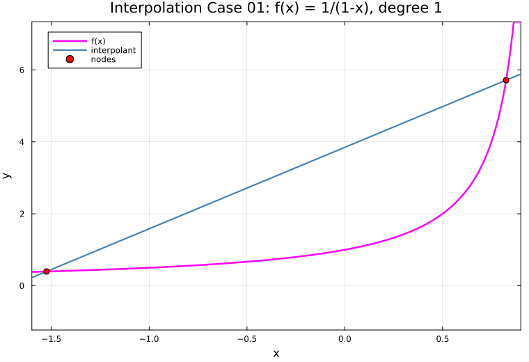
Case 01
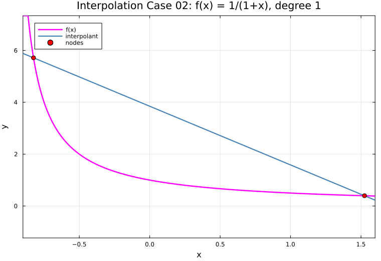
Case 02
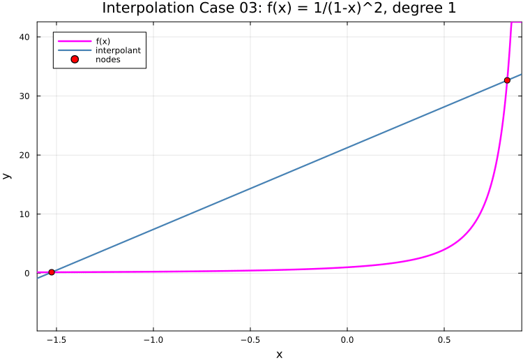
Case 03
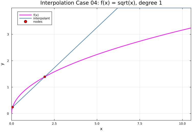
Case 04
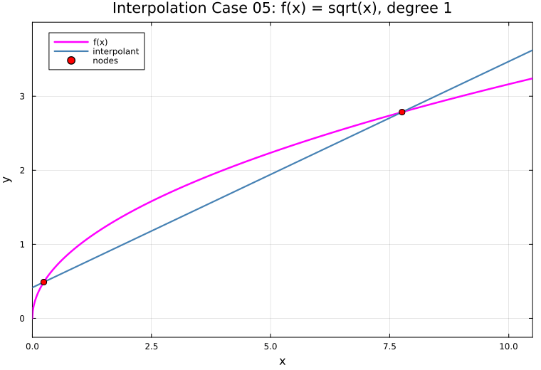
Case 05
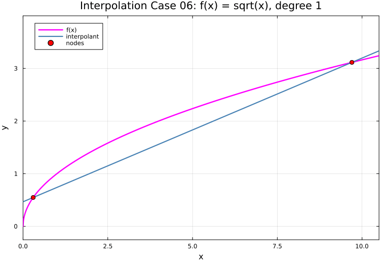
Case 06
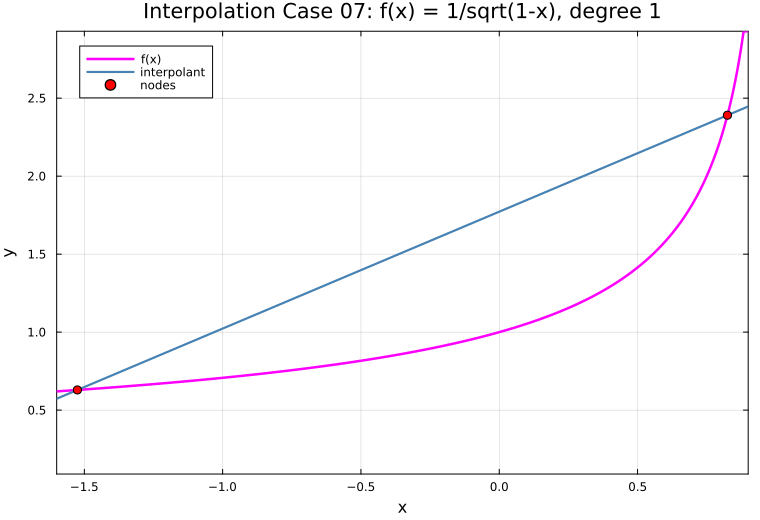
Case 07
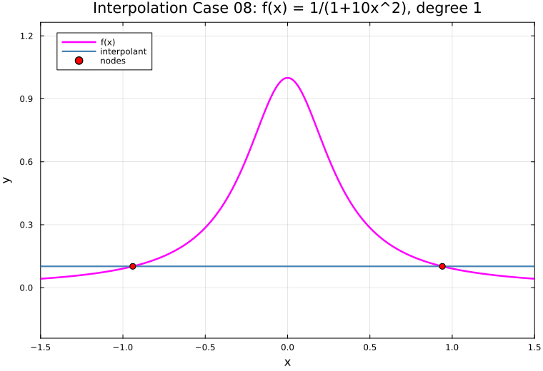
Case 08
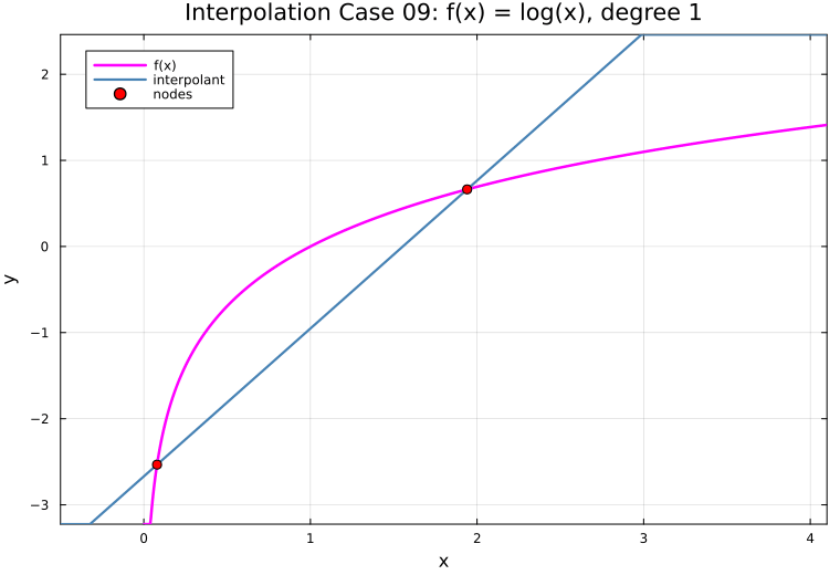
Case 09
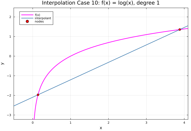
Case 10
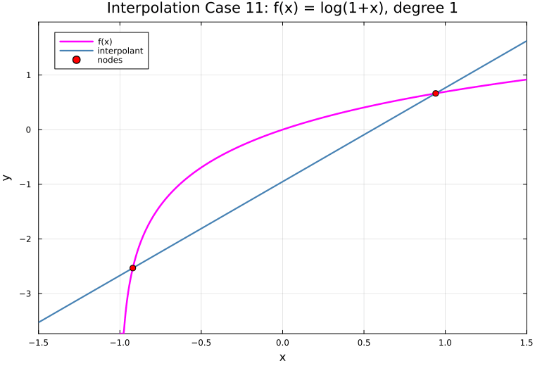
Case 11
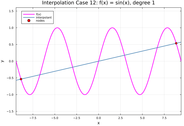
Case 12
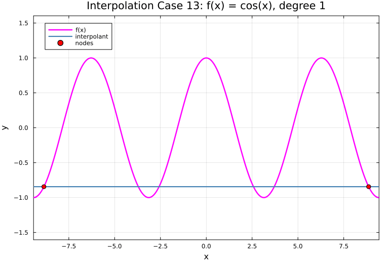
Case 13
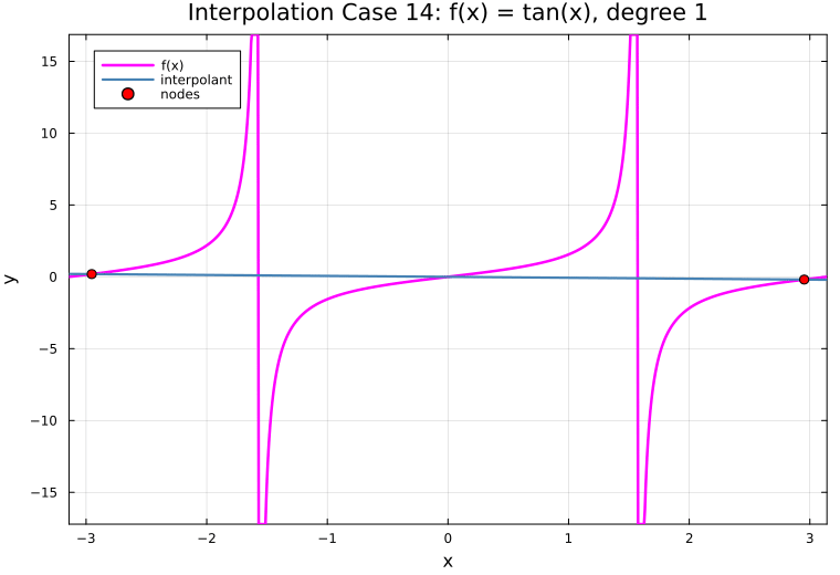
Case 14
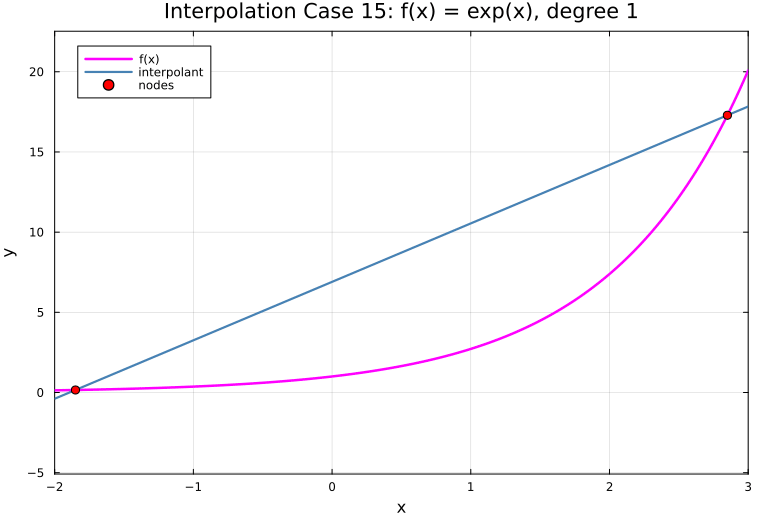
Case 15
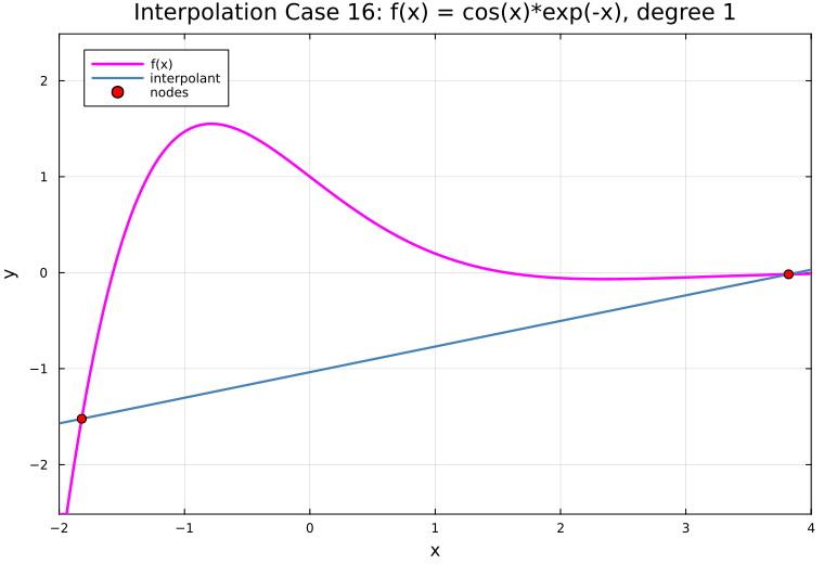
Case 16
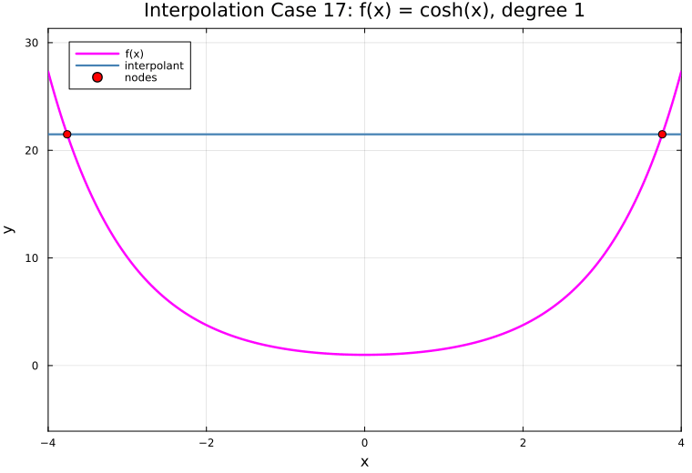
Case 17
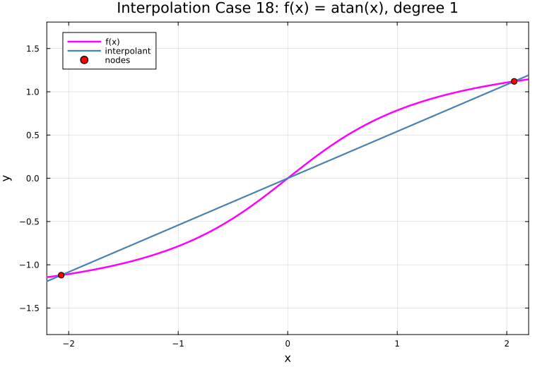
Case 18
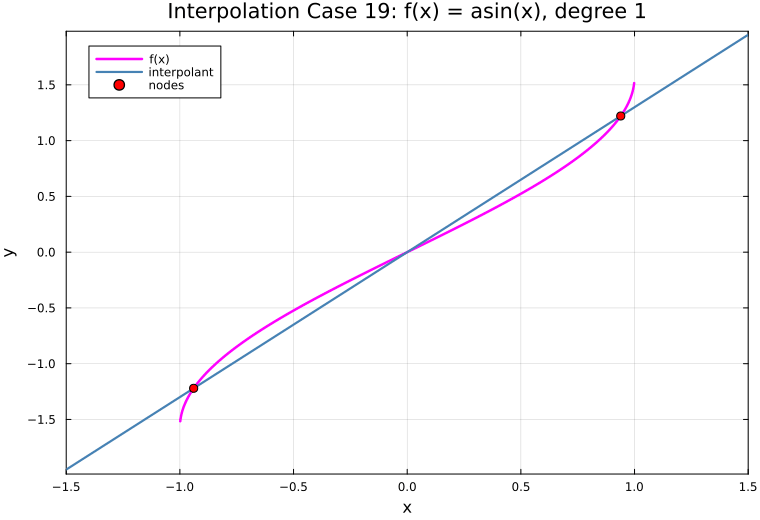
Case 19
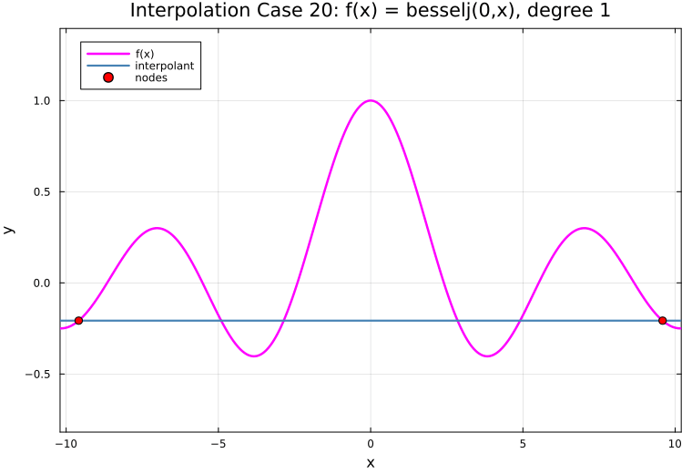
Case 20
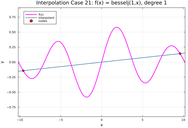
Case 21
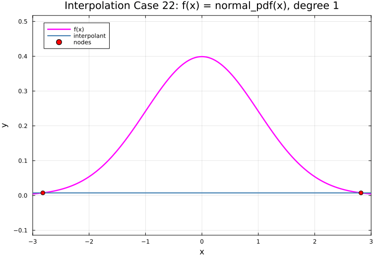
Case 22
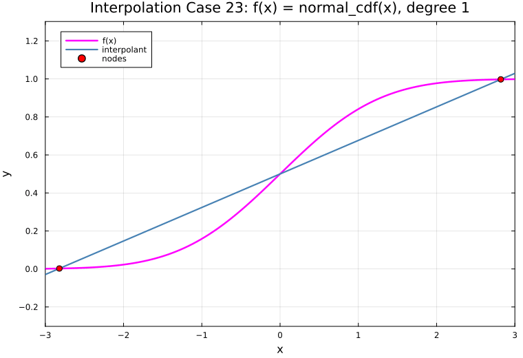
Case 23
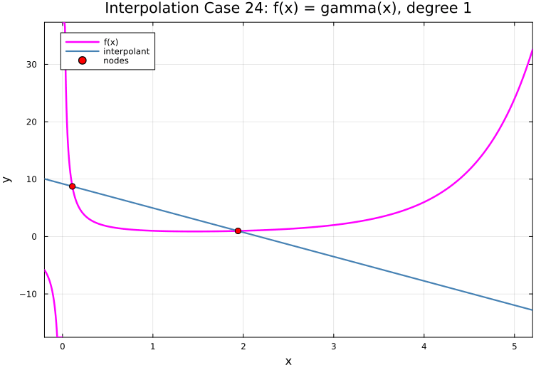
Case 24
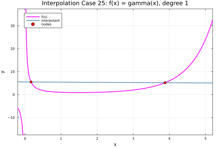
Case 25
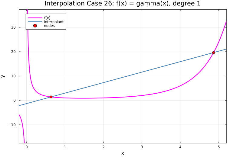
Case 26
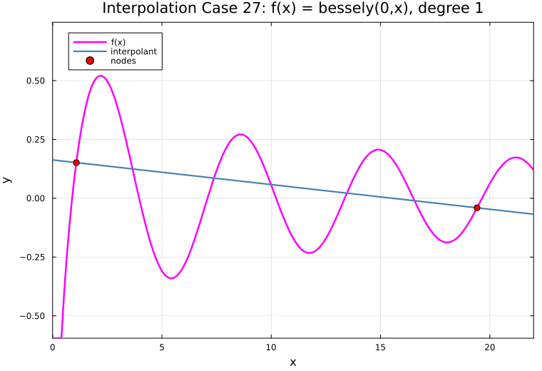
Case 27
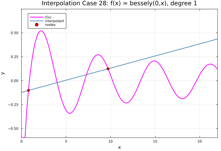
Case 28
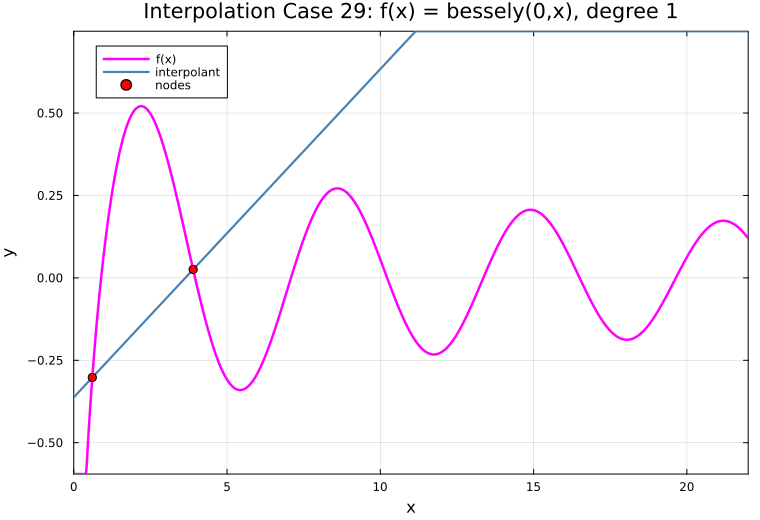
Case 29
Derivation Notes (Planned)
Short derivations will be added for divided differences, nested evaluation, and incremental updates.
References
Mathew, John H. 2000-2019. Numerical Analysis - Numerical Methods Modules. https://web.archive.org/web/20190808102217/http://mathfaculty.fullerton.edu/mathews/n2003/NumericalUndergradMod.html.