Legendre Polynomials
Source inspiration: (Mathew 2000-2019).
Animations
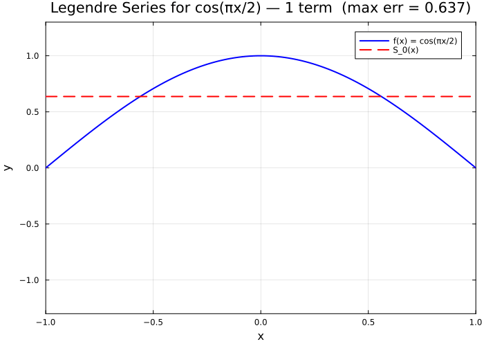
Each animation below illustrates Legendre polynomials \(P_n(x)\) on \([-1,1]\). The first animation reveals \(P_0\) through \(P_5\) one per frame; the second shows the Legendre series partial sums converging to \(f(x) = \cos(\pi x/2)\).
Julia source scripts that generated these animations are linked under each case.
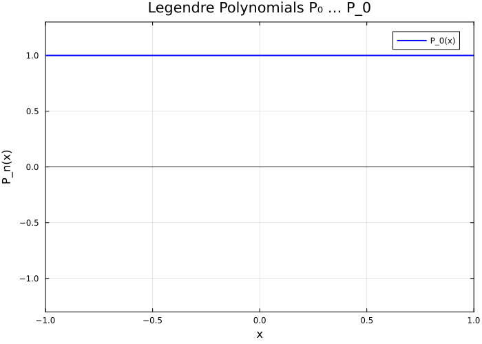
Case 1 — Successive polynomials \(P_0, P_1, \ldots, P_5\)
Properties: Each \(P_n\) is orthogonal to all lower-degree Legendre polynomials on \([-1,1]\). \(P_n(1)=1\), \(P_n(-1)=(-1)^n\), and \(P_n\) has exactly \(n\) zeros in \((-1,1)\). They are computed by the recurrence \((n+1)P_{n+1} = (2n+1)xP_n - nP_{n-1}\).
Case 2 — Legendre series for \(f(x) = \cos(\pi x/2)\)
Behavior: The partial sum \(S_N(x) = \sum_{n=0}^{N} c_n P_n(x)\) with \(c_n = \tfrac{2n+1}{2}\int_{-1}^{1} f(x)P_n(x)\,dx\) converges to \(f\) as \(N\to\infty\). Only even-\(n\) terms contribute (since \(f\) is even). Each added term refines the fit.